Categorical Data - Contingency Tables

Introduction to Global Health Data Science

Prof. Amy Herring

Duke University
STA/GLHLTH 198 Fall 2026

Introduction to contingency tables

Motivating example: Streptococcus pneumoniae

Infections due to Streptococcus pneumoniae remain a substantial source of morbidity and mortality in both developing and developed countries despite a century of research and the development of therapeutic interventions such as multiple classes of antibiotics and vaccination. The World Health Organization estimates that in developing countries 814,000 children under the age of five die annually from invasive pneumococcal disease (IPD), with an estimated 1.6 million deaths affecting all ages globally.

Several recent studies have identified associations between pneumococcal serotypes (species variations) and patient outcomes from IPD. We consider data from a Scottish study of pneumococcal serotypes and mortality.

Contingency tables

A contingency table is a display format for showing the relationship between two categorical variables. Below is a contingency table for a subset of serotypes from the Scottish study.

Serotype	Survived	Died	Total
Serotype 10	37	7	44
Serotype 15	60	12	72
Serotype 20	97	9	106
Serotype 31	24	10	34
Total	218	38	256

Dataset (Random sample of observations printed)

Serotype	Survived
Serotype 10	Survived
Serotype 15	Survived
Serotype 31	Did not survive
Serotype 20	Survived
Serotype 15	Survived
Serotype 31	Survived
Serotype 15	Did not survive
Serotype 20	Survived
Serotype 20	Survived
Serotype 20	Survived
Serotype 20	Survived
Serotype 20	Survived
Serotype 15	Survived
Serotype 15	Survived
Serotype 20	Did not survive
Serotype 15	Survived
Serotype 15	Survived
Serotype 15	Survived
Serotype 20	Survived
Serotype 15	Did not survive

Visualizing Serotypes and Survival

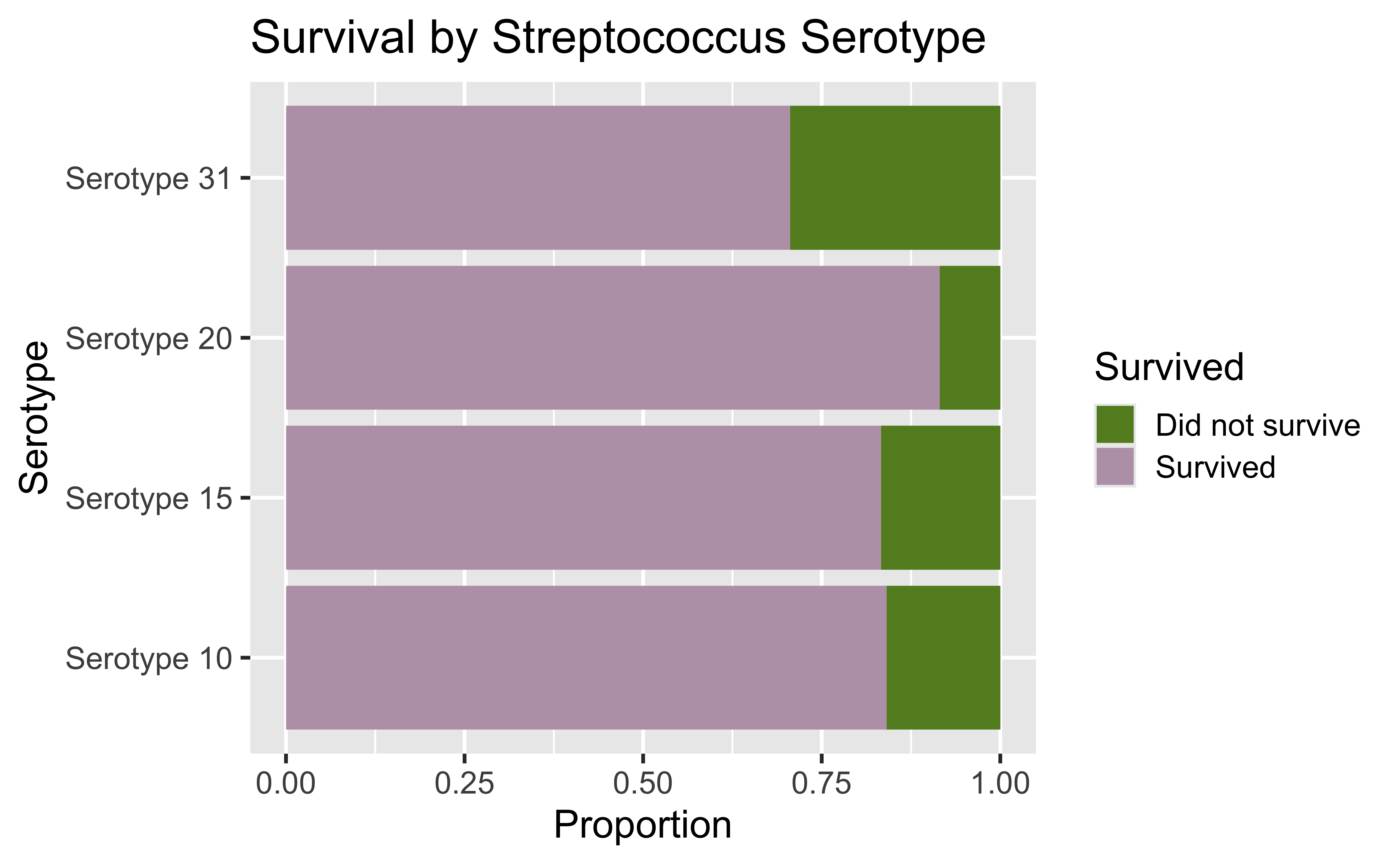
Here’s the relationship in the sample data.

• Plot
• Code

pneu %>%
  ggplot(aes(y = Serotype, fill = Survived)) +
  geom_bar(position = "fill") +
  labs(x="Proportion",
       title="Survival by Streptococcus Serotype") + 
  scale_fill_manual(values=c("#638B27","#BBA2B6"))

Are serotype and survival related?

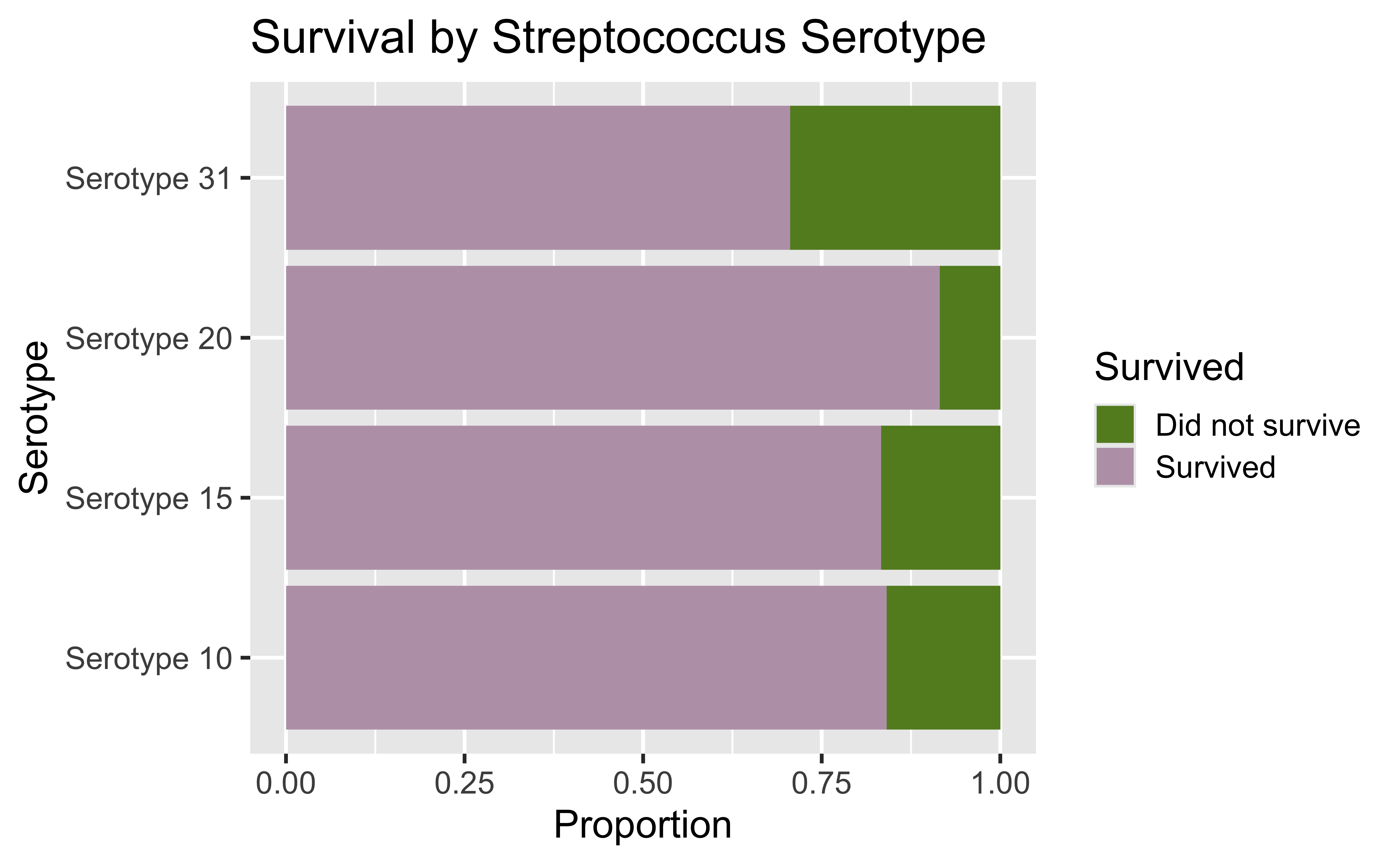
If there were no relationship between serotype and survival, we’d expect to see the lavender bars all the same length across the serotypes. Are the differences we see here reflecting actual differences in population-level survival across serotypes, or are they just a function of random variation?

Typical questions of interest with \(r \times c\) contingency tables

• Is there an association between the row variable (indexed by \(r\)) and the column variable (indexed by \(c\))?

  • In our case, \(r=4\) (4 serotypes) and \(c=2\) (survived or died). We could easily reverse rows and columns with no ill effects.

• How strong is any association?

Here, we would like to test \(H_0:\) pneumococcal serotype is unrelated to mortality against the alternative \(H_A:\) pneumococcal serotype is related to mortality

Tests for Association

Fisher’s Exact Test

Fisher’s Exact Test

Fisher’s exact test is a great first choice for testing a relationship between two variables in a contingency table. While it has been around for almost 100 years, it was originally used only for very small samples due to the computational burden involved (this concern has been largely alleviated by modern computing). This test was invented by the same person for whom the F test we studied recently was named (Fisher made many important contributions to statistics).

Fisher’s Exact Test

Fisher’s exact test is fairly intuitive. The way it works is that we assume the column and row totals are fixed (so for our pneumococcus example, we condition on having 38 deaths and 218 survivors and that we have 34 in serotype 31, 44 in serotype 10, 72 in serotype 15, and 106 in serotype 20). Then, we construct all possible contingency tables with the same margins, and then sum up the probabilities of all tables with null probabilities less than or equal to that of our observed table to get the p-value (recall the p-value is the probability of the observed data, or more extreme data, occurring under the null hypothesis).

Margins: row and column totals

Obviously, this was no fun before modern computing.

Tables with the same margins

Our table:

Serotype	Survived	Died	Total
Serotype 10	37	7	44
Serotype 15	60	12	72
Serotype 20	97	9	106
Serotype 31	24	10	34
Total	218	38	256

A more extreme table with same margins:

Serotype	Survived	Died	Total
Serotype 10	38	6	44
Serotype 15	60	12	72
Serotype 20	97	9	106
Serotype 31	23	11	34
Total	218	38	256

A more extreme table

Our table:

Serotype	Survived	Died	Total
Serotype 10	37	7	44
Serotype 15	60	12	72
Serotype 20	97	9	106
Serotype 31	24	10	34
Total	218	38	256

A more extreme table with same margins:

Serotype	Survived	Died	Total
Serotype 10	44	0	44
Serotype 15	60	12	72
Serotype 20	97	9	106
Serotype 31	17	17	34
Total	218	38	256

Conducting the test for Pneumococcus data

fisher.test(pneu$Serotype,pneu$Survived)

#> 
#>  Fisher's Exact Test for Count Data
#> 
#> data:  pneu$Serotype and pneu$Survived
#> p-value = 0.02658
#> alternative hypothesis: two.sided

Here we conclude that the rows and columns of our table are not independent. That is, we conclude that there is a relationship between serotype and survival.

\(\chi^2\) (Chi-Squared) Test

\(\chi^2\) Test

We can also test our null hypothesis that serotype is unrelated to survival using a \(\chi^2\) test.

The chi-squared approximation depends on the expected cell counts under \(H_0\). For this course, use the guideline that every expected cell count should be at least 5. Fisher’s exact test does not require large expected counts.

Yates’ continuity correction applies to \(2\times2\) tables. In R, chisq.test() uses it by default for those tables. It does not apply to our \(4\times2\) table.

For very large samples, Fisher’s exact test can still be too computationally expensive, and the \(\chi^2\) test has nice connections to the logistic regression models we will study later in the course.

In addition, the chi-squared test has a very nice motivation in terms of comparing observed proportions in the data to the proportions we would expect if \(H_0\) were true.

The source notes used observed counts greater than 10 and described Yates’ correction as a response to small counts. The relevant quantities are expected counts, and R applies the continuity correction by default only to 2 x 2 tables. See the R documentation: https://stat.ethz.ch/R-manual/R-devel/library/stats/html/chisq.test.html https://stat.ethz.ch/R-manual/R-devel/library/stats/html/fisher.test.html

Marginal probabilities

table(pneu$Serotype, pneu$Survived) %>%
  knitr::kable()

	Did not survive	Survived
Serotype 10	7	37
Serotype 15	12	60
Serotype 20	9	97
Serotype 31	10	24

Some summaries of marginal probabilities will be helpful as we consider the data.

Survived: \(\frac{37+60+97+24}{37+60+97+24+7+12+9+10}=\frac{218}{256}=85.2\%\) survived

Prevalence of serotypes: serotype 10: \(\frac{44}{256}=17.2\%\); serotype 15: \(\frac{72}{256}=28.1\%\); serotype 20: \(\frac{106}{256}=41.4\%\); serotype 31: \(\frac{34}{256}=13.3\%\)

\(\chi^2\) Test

Suppose that \(H_0\) is true, and serotype of infection and survival are independent events. In that case, how would we calculate the probability that a patient had serotype 10 and survived?

Back to probability!

Remember for two independent events, \(P(A \cap B)=P(A)P(B)\).

Another handy probability law in this setting is the law of total probability, e.g. \(P(A)+P(A^c)=1\).

We can use these probability rules to calculate what our table would be expected to look like, given fixed margins (i.e., the same number of survivors and infections of each serotype as we have here), if \(H_0\) is true. When \(H_0\) is true, the serotype is independent of survival.

\(\chi^2\) Test

Let’s create the table we would expect to see if \(H_0\) were true.

? = expected # who survived and had serotype 10 if \(H_0\) true

? = probability of being both serotype 10 and surviving times number of study participants = P(Serotype 10) \(\times\) P(Survived) \(\times\) 256

? = \(\frac{44}{256}\times\frac{218}{256}\times 256=37.5\)

	Survived	Died	Total
Serotype 10	?		44
Serotype 15			72
Serotype 20			106
Serotype 31			34
Total	218	38	256

\(\chi^2\) Test

? can be obtained by subtraction as 44-37.5

	Survived	Died	Total
Serotype 10	37.5	?	44
Serotype 15			72
Serotype 20			106
Serotype 31			34
Total	218	38	256

\(\chi^2\) Test

? = expected # who survived and had serotype 15 if \(H_0\) true

? = probability of being both serotype 15 and surviving times number of study participants = P(Serotype 15) \(\times\) P(Survived) \(\times\) 256

? = \(\frac{72}{256}\times\frac{218}{256}\times 256=61.3\)

	Survived	Died	Total
Serotype 10	37.5	6.5	44
Serotype 15	?		72
Serotype 20			106
Serotype 31			34
Total	218	38	256

\(\chi^2\) Test

? can be obtained by subtraction as 72-61.3

	Survived	Died	Total
Serotype 10	37.5	6.5	44
Serotype 15	61.3	?	72
Serotype 20			106
Serotype 31			34
Total	218	38	256

\(\chi^2\) Test

? = expected # who survived and had serotype 20 if \(H_0\) true

? = probability of being both serotype 20 and surviving times number of study participants = P(Serotype 20) \(\times\) P(Survived) \(\times\) 256

? = \(\frac{106}{256}\times\frac{218}{256}\times 256=90.3\)

The remainder of the entries in the table can be obtained now by subtraction.

	Survived	Died	Total
Serotype 10	37.5	6.5	44
Serotype 15	61.3	10.7	72
Serotype 20	?		106
Serotype 31			34
Total	218	38	256

\(\chi^2\) Test

	Survived	Died	Total
Serotype 10	37.5	6.5	44
Serotype 15	61.3	10.7	72
Serotype 20	90.3	106-90.3	106
Serotype 31			34
Total	218	38	256

\(\chi^2\) Test

	Survived	Died	Total
Serotype 10	37.5	6.5	44
Serotype 15	61.3	10.7	72
Serotype 20	90.3	15.7	106
Serotype 31	\(34\times\frac{218}{256}\)		34
Total	218	38	256

\(\chi^2\) Test

	Survived	Died	Total
Serotype 10	37.5	6.5	44
Serotype 15	61.3	10.7	72
Serotype 20	90.3	15.7	106
Serotype 31	29.0	\(34-34\times\frac{218}{256}\)	34
Total	218	38	256

\(\chi^2\) Test

Thus if \(H_0\) is true, we would expect to see a table like this. Expected counts are calculated at full precision and then rounded to one decimal place.

	Survived	Died	Total
Serotype 10	37.5	6.5	44
Serotype 15	61.3	10.7	72
Serotype 20	90.3	15.7	106
Serotype 31	29.0	5.0	34
Total	218	38	256

Comparing Observed and Expected Tables

Observed Table

Serotype	Survived	Died	Total
Serotype 10	37	7	44
Serotype 15	60	12	72
Serotype 20	97	9	106
Serotype 31	24	10	34
Total	218	38	256

Expected Table under \(H_0\)

	Survived	Died	Total
Serotype 10	37.5	6.5	44
Serotype 15	61.3	10.7	72
Serotype 20	90.3	15.7	106
Serotype 31	29.0	5.0	34
Total	218	38	256

So we do observe some different proportions than we would expect under \(H_0\), in particular for serotypes 20 and 31. Is this “different enough” for us to raise an alarm about one or more serotypes?

Comparing Observed and Expected Tables

Observed Table

Serotype	Survived	Died	Total
Serotype 10	37	7	44
Serotype 15	60	12	72
Serotype 20	97	9	106
Serotype 31	24	10	34
Total	218	38	256

Expected Table under \(H_0\)

	Survived	Died	Total
Serotype 10	37.5	6.5	44
Serotype 15	61.3	10.7	72
Serotype 20	90.3	15.7	106
Serotype 31	29.0	5.0	34
Total	218	38	256

• The \(\chi^2\) test compares the observed frequencies, \(O\), in each cell of the table to the expected frequencies, \(E\), if \(H_0\) is true.

Comparing Observed and Expected Tables

Observed Table

Serotype	Survived	Died	Total
Serotype 10	37	7	44
Serotype 15	60	12	72
Serotype 20	97	9	106
Serotype 31	24	10	34
Total	218	38	256

Expected Table under \(H_0\)

	Survived	Died	Total
Serotype 10	37.5	6.5	44
Serotype 15	61.3	10.7	72
Serotype 20	90.3	15.7	106
Serotype 31	29.0	5.0	34
Total	218	38	256

• If differences between what we observe and expect, \(O-E\), are large enough, we reject \(H_0\).

Comparing Observed and Expected Tables

Observed Table

Serotype	Survived	Died	Total
Serotype 10	37	7	44
Serotype 15	60	12	72
Serotype 20	97	9	106
Serotype 31	24	10	34
Total	218	38	256

Expected Table under \(H_0\)

	Survived	Died	Total
Serotype 10	37.5	6.5	44
Serotype 15	61.3	10.7	72
Serotype 20	90.3	15.7	106
Serotype 31	29.0	5.0	34
Total	218	38	256

• To combine differences across table cells, we need to square them (so that extra deaths in one serotype are not cancelled out by fewer deaths in another serotype) before adding them up.

Comparing Observed and Expected Tables

Observed Table

Serotype	Survived	Died	Total
Serotype 10	37	7	44
Serotype 15	60	12	72
Serotype 20	97	9	106
Serotype 31	24	10	34
Total	218	38	256

Expected Table under \(H_0\)

	Survived	Died	Total
Serotype 10	37.5	6.5	44
Serotype 15	61.3	10.7	72
Serotype 20	90.3	15.7	106
Serotype 31	29.0	5.0	34
Total	218	38	256

• In addition, we need to scale the differences. That is, seeing 5 ‘extra’ deaths is a big deal if our study only contains 10 participants and is not a big deal if our study contains 100,000 participants, so we divide by \(E\) to examine relative differences

Comparing Observed and Expected Tables

Observed Table

Serotype	Survived	Died	Total
Serotype 10	37	7	44
Serotype 15	60	12	72
Serotype 20	97	9	106
Serotype 31	24	10	34
Total	218	38	256

Expected Table under \(H_0\)

	Survived	Died	Total
Serotype 10	37.5	6.5	44
Serotype 15	61.3	10.7	72
Serotype 20	90.3	15.7	106
Serotype 31	29.0	5.0	34
Total	218	38	256

Our test statistic is \(X^2=\sum_{i=1}^{rc} \frac{(O_i-E_i)^2}{E_i},\) where \(r\times c=rc\) is the number of cells in the table (not including any totals, so there are 8 cells here). So here that’s \[\frac{(37-37.5)^2}{37.5}+\frac{(7-6.5)^2}{6.5}+ \cdots + \frac{(10-5.0)^2}{5.0}\]

\(\chi^2\) Test

• The distribution of this sum is approximated by a chi-squared distribution with \((r-1)(c-1)\) degrees of freedom, written \({\chi^2}_{(r-1)(c-1)}\)

• Like the \(F\) distribution, there is a different \(\chi^2\) distribution for each degrees of freedom, and chi-squared distribution is not symmetric

• Like the \(F\) distribution, all the mass is above 0, and to calculate the p-value we look at the area in the right tail only.

\(\chi^2\) Statistic

observed_chisq_statistic <- pneu %>%
  specify(Serotype ~ Survived) %>%
  calculate(stat = "Chisq")

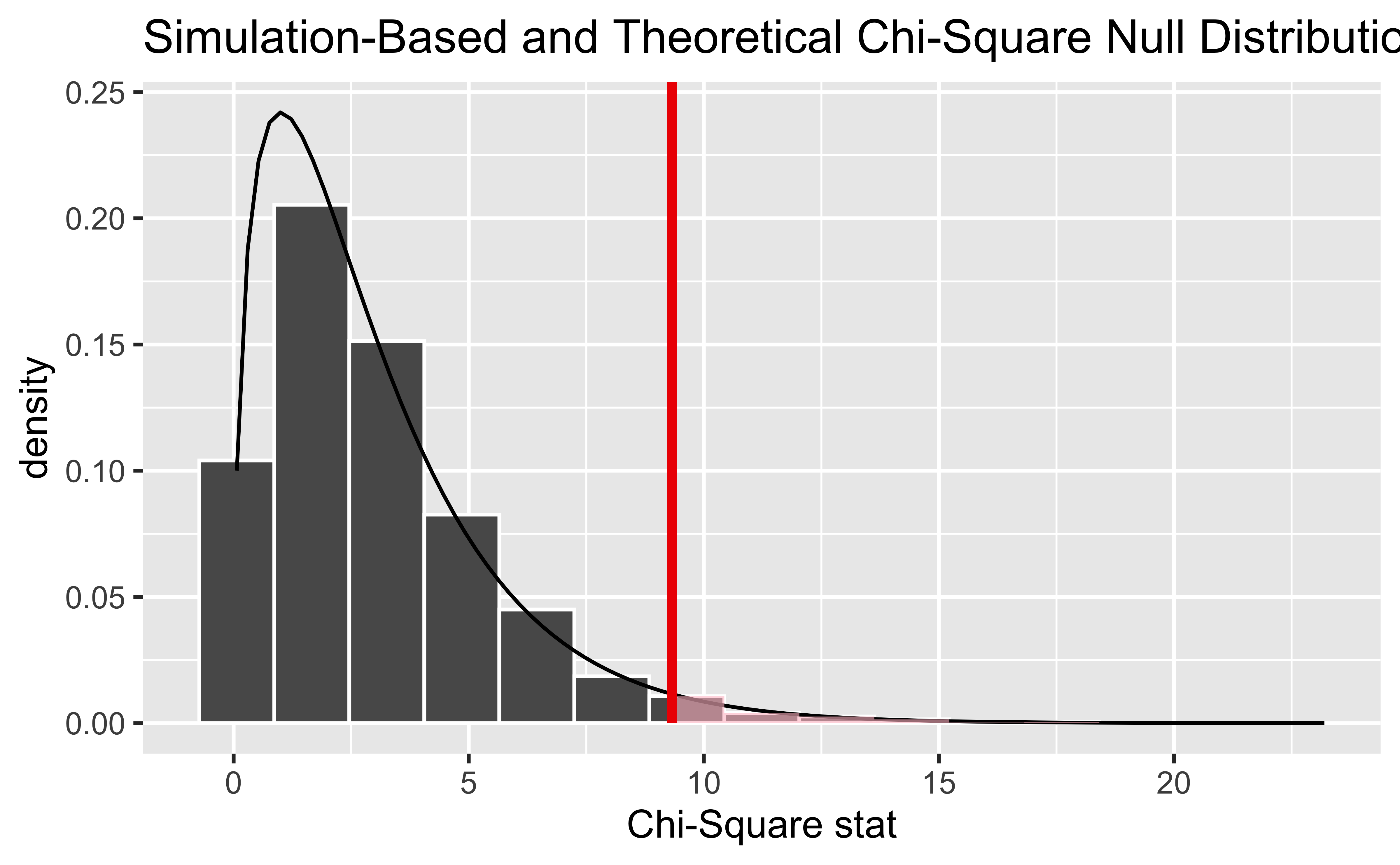
Before we calculate the p-value corresponding to this test statistic, we can visualize the distribution of \(\chi^2_{(4-1)(2-1)}=\chi^2_3\) statistics we would see under \(H_0\).

Simulating the null distribution

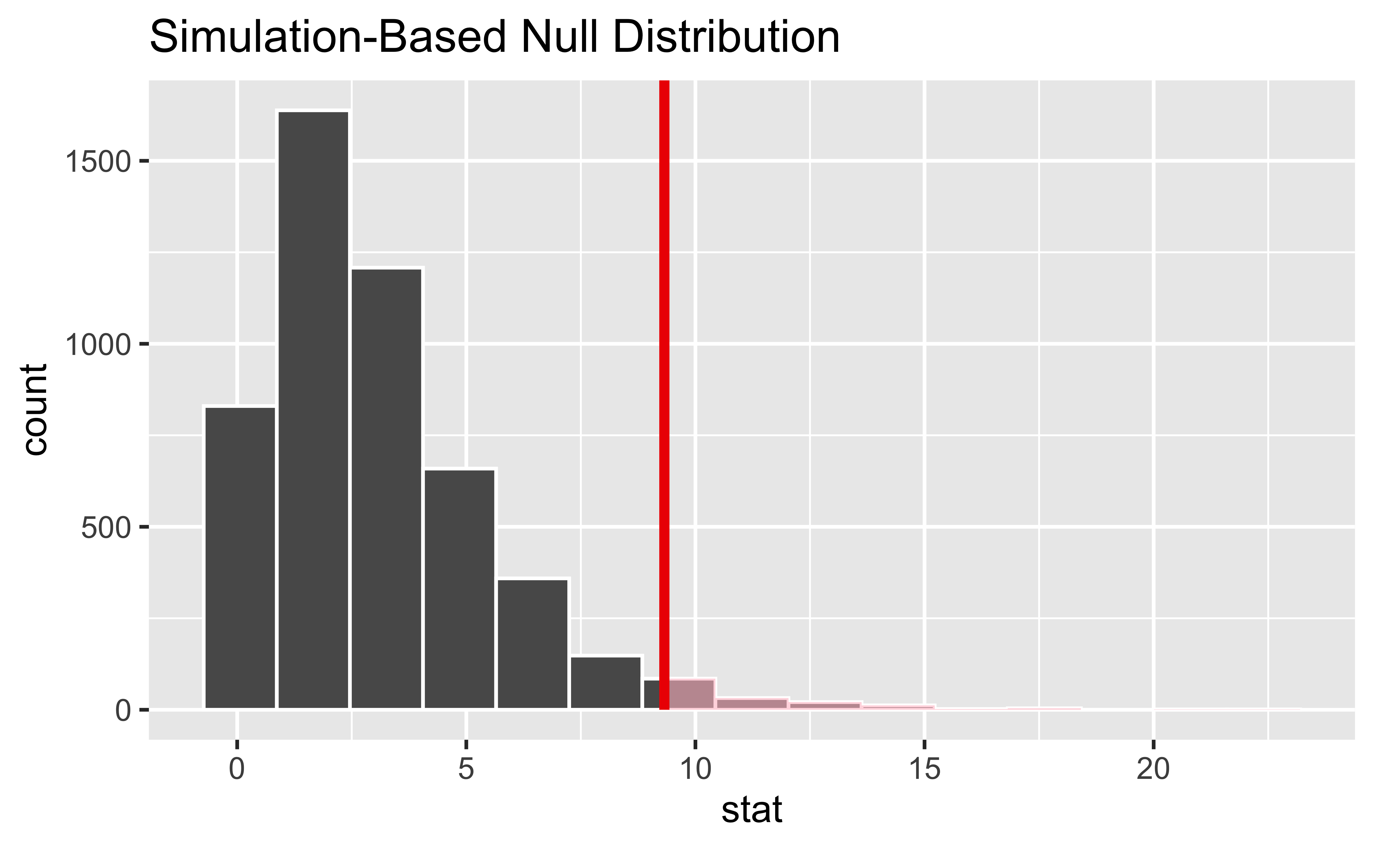
We can visualize the null distribution in two ways: by looking at the \(\chi^2_3\) distribution directly or by randomly sampling to generate the null distribution. First, let’s consider a simulated null distribution.

# generate the null distribution using randomization
null_distribution_simulated <- pneu %>%
  specify(Serotype ~ Survived) %>%
  hypothesize(null = "independence") %>%
  generate(reps = 5000, type = "permute") %>%
  calculate(stat = "Chisq")

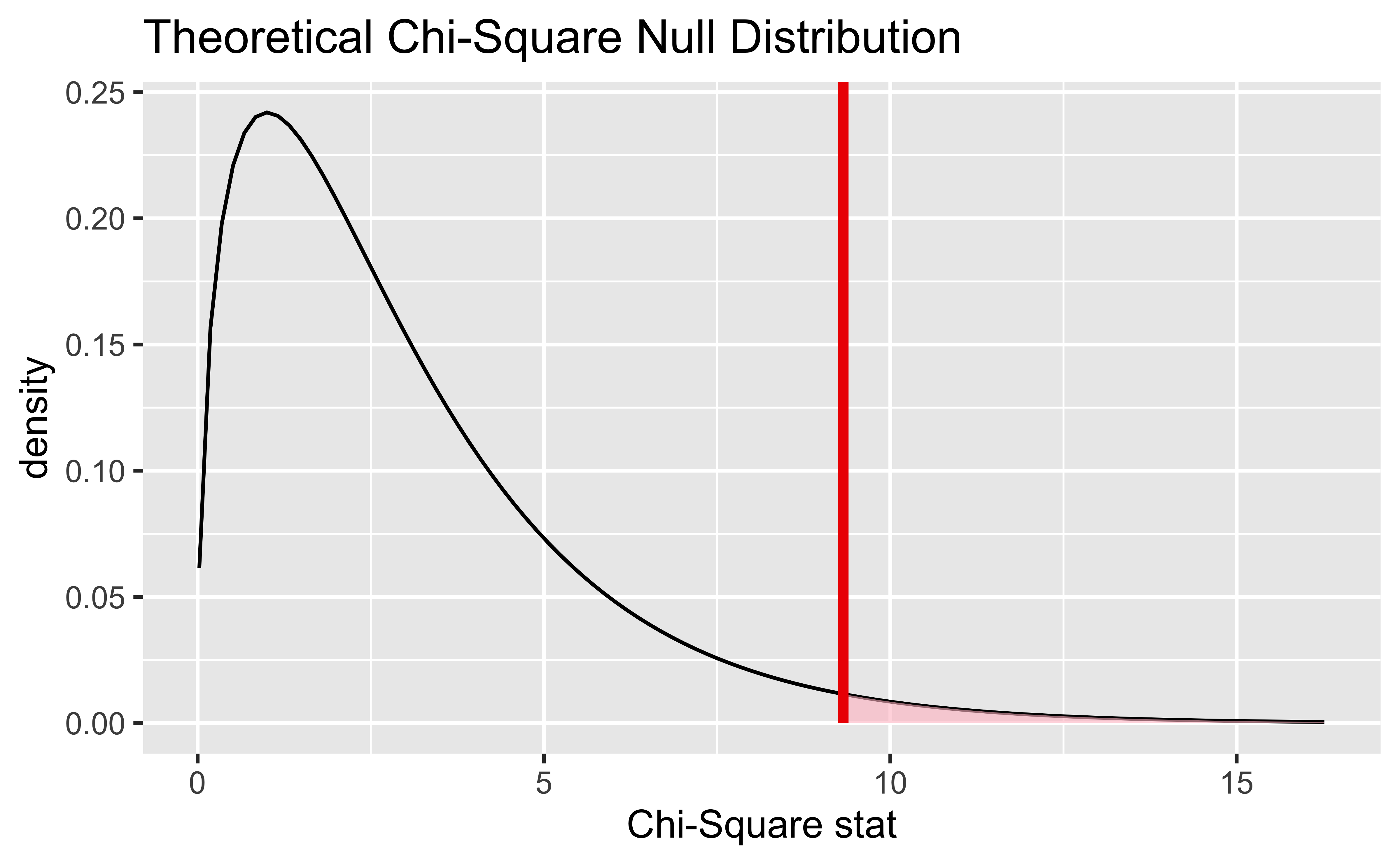
The theoretical null distribution

Next we can use the \(\chi^2_3\) distribution as an approximation to the null distribution.

# Specify the test for use with the theoretical approximation.
null_distribution_theoretical <- pneu %>%
  specify(Serotype ~ Survived) %>%
  hypothesize(null = "independence") %>%
# No permutation generation is needed for the theoretical approximation.
  calculate(stat = "Chisq")

Visualizing the simulated null distribution

Let’s visualize based on the simulated null distribution.

• Plot
• Code

# visualize the null distribution and test statistic!
null_distribution_simulated %>%
  visualize() + 
  shade_p_value(observed_chisq_statistic,
                direction = "greater")

Visualizing the theoretical null distribution

We can also visualize based on the theoretical distribution, \(\chi^2_3\).

• Plot
• Code

# visualize the theoretical null distribution and test statistic!
pneu %>%
  specify(Serotype ~ Survived) %>%
  hypothesize(null= "independence") %>%
  visualize(method = "theoretical") + 
  shade_p_value(observed_chisq_statistic,
                direction = "greater")

Comparing both null distributions

Here we can also have our cake and eat it, too! Let’s visualize both.

• Plot
• Code

# visualize both null distributions and the test statistic!
null_distribution_simulated %>%
  visualize(method = "both") + 
  shade_p_value(observed_chisq_statistic,
                direction = "greater")

Conducting the chi-squared test

We can now carry out the test.

chisq_test(pneu,Serotype~Survived)

#> # A tibble: 1 × 3
#>   statistic chisq_df p_value
#>       <dbl>    <int>   <dbl>
#> 1      9.32        3  0.0253

If there were no relationship, the probability we would see a \(\chi^2_3\) test statistic as large as 9.32 or larger is just 0.0253. So serotypes are related to survival probability.

Step-Down Tests

We can also compare pairs of serotypes. If we test multiple pairs, we should adjust for multiple comparisons before concluding which serotypes differ. Here, we compare serotypes 20 and 31.

pneu2 <- pneu %>%
  filter(Serotype=="Serotype 20" | Serotype == "Serotype 31")
chisq_test(pneu2,Serotype~Survived)

#> # A tibble: 1 × 3
#>   statistic chisq_df p_value
#>       <dbl>    <int>   <dbl>
#> 1      7.91        1 0.00493

How strong is the association?

The Odds Ratio (OR)

Suppose we have a disease \(D\) (e.g., lung cancer) and two groups, \(E\) and \(E^c\), where \(E\)=smokers and \(E^c\)=nonsmokers.

\[OR=\frac{\left\{\frac{Pr(D \mid E)}{1-Pr(D \mid E)}\right\}}{\left\{\frac{Pr(D \mid E^c)}{1-Pr(D \mid E^c)}\right\}}\]

The OR ranges from 0 to \(\infty\). When \(OR=1\) (even odds), there is no association between two variables.

Odds Ratio

Consider the following contingency table.

	Exposed	Unexposed	Total
Disease	a	b	a+b
No disease	c	d	c+d
Total	a+c	b+d	a+b+c+d

\[\widehat{Pr}(D \mid E)=\frac{a}{a+c}\] \[\widehat{Pr}(D \mid E^c) = \frac{b}{b+d}\]

Odds Ratio

\[\widehat{Pr}(D \mid E)=\frac{a}{a+c} ~~~~~~~\widehat{Pr}(D \mid E^c) = \frac{b}{b+d}\] \[OR=\frac{\left\{\frac{Pr(D \mid E)}{1-Pr(D \mid E)}\right\}}{\left\{\frac{Pr(D \mid E^c)}{1-Pr(D \mid E^c)}\right\}}\]

\[\widehat{OR}=\frac{\left\{\frac{\frac{a}{a+c}}{\frac{c}{a+c}}\right\}}{\left\{\frac{\frac{b}{b+d}}{\frac{d}{b+d}} \right\}} =\frac{ad}{bc}\]

Estimating an OR and a 95% CI for it

Many R packages will estimate an odds ratio and 95% CI for it when provided a 2 \(\times\) 2 table. For now, we can take advantage of the fact that the fisher.test function does this automatically. First, though, we need to subset to only two serotypes. Below we subset to serotypes 20 and 31 so we get an OR comparing these two. Our null hypothesis is that the survival probabilities are the same for both serotypes, and the alternative is that they are different.

pneu2 <- pneu %>%
  filter(Serotype=="Serotype 20" | Serotype == "Serotype 31")

Odds ratio: serotype 20 versus serotype 31

table(pneu2$Serotype, pneu2$Survived)

#>              
#>               Did not survive Survived
#>   Serotype 20               9       97
#>   Serotype 31              10       24

# Columns are ordered: Did not survive, Survived.
# The OR compares odds of death for serotype 20 versus serotype 31.
fisher.test(table(pneu2$Serotype, pneu2$Survived))

#> 
#>  Fisher's Exact Test for Count Data
#> 
#> data:  table(pneu2$Serotype, pneu2$Survived)
#> p-value = 0.003891
#> alternative hypothesis: true odds ratio is not equal to 1
#> 95 percent confidence interval:
#>  0.07201804 0.69330783
#> sample estimates:
#> odds ratio 
#>  0.2257481

\(\widehat{OR}=0.23\) with a 95% CI of (0.07, 0.69). Those infected with serotype 20 have just 0.23 (95% CI=(0.07, 0.69)) times the odds of death as those infected with serotype 31.

Comparing serotypes 10 and 31

Now we can quantify other differences. For example, we may wish to evaluate whether serotype 10 and serotype 31 have the same survival probability or not.

pneu3 <- pneu %>%
  filter(Serotype=="Serotype 10" | Serotype == "Serotype 31")
table(pneu3$Serotype, pneu3$Survived)

#>              
#>               Did not survive Survived
#>   Serotype 10               7       37
#>   Serotype 31              10       24

Fisher’s exact test: serotypes 10 and 31

fisher.test(table(pneu3$Serotype, pneu3$Survived))

#> 
#>  Fisher's Exact Test for Count Data
#> 
#> data:  table(pneu3$Serotype, pneu3$Survived)
#> p-value = 0.1758
#> alternative hypothesis: true odds ratio is not equal to 1
#> 95 percent confidence interval:
#>  0.128805 1.546707
#> sample estimates:
#> odds ratio 
#>    0.45881

What do you conclude?