Discrete Probability Distributions

Introduction to Global Health Data Science

Amy Herring

Duke University
STA/GLHLTH 198 Fall 2026

2026-09-09

Probability Distributions

When we learned how to find probabilities using basic principles, we focused on one particular outcome or event, like the probability of a randomly selected person being left-handed. We now explore the bigger picture by exploring all possible values of a discrete random variable, along with their associated probabilities. This list of possible values and probabilities is called the probability distribution of the random variable.

Why do we care about probability distributions?

We need probability distributions to make statements about how likely an event may be.

For example, suppose we are interested in comparing two groups of pancreatic cancer patients, with one group on the standard treatment and one group on an experimental new treatment.

The statistical test we use to compare the two groups depends on the variable of interest $X$ and its probability distribution.

Why do we care about probability distributions?

Possible outcomes for comparison:

define $X$ to be a 0/1 variable indicating whether each patient survives 1 year
define $X$ as the number of months a patient survives

In these two cases, under each definition, $X$ has a different probability distribution, and you would use a different type of test for each case.

Example: Y Chromosomes

Consider Y chromosomes in the US population. Roughly 51.2% of births are of babies with Y chromosomes, and 48.8% of babies do not have Y chromosomes. Thus the probability of having a baby with a Y chromosome is 0.512.

The probability of an event is $\geq 0$ and $\leq 1$.
The sum of the probabilities of all possible events is exactly 1 (e.g., 0.512+0.488=1).
So the probability of having a baby without a Y chromosome is 0.488.

Note: sex ratios vary dramatically across species, driven by factors including environmental sex determination (nest temperature in sea turtles), mating systems (bluestreak cleaner wrasse have no primary males), and social structure (ants and bees)

Bernoulli Distribution

Consider a dichotomous (two-level) random variable $Y$. By definition, $Y$ must assume one of two possible values, e.g.

failure or success
Y chromosome present or not
Duke student or not
current smoker or not
heads or tails (coin flip)

A random variable of this type is known as a Bernoulli random variable, and we describe the probability of response using the parameter $\pi$.

The distribution is named for Jacob Bernoulli, who was part of a famous family of mathematicians in Switzerland.

Bernoulli random variable

These variables are often coded so that $Y=1$ is called the event or a success, $Y=0$ is called a failure, and $\pi$ is defined as the probability of a success. (This is not required, but you need to remember which level maps to $\pi$, and the other level then has probability $1-\pi$.)

Bernoulli random variable examples

Coin flip: let $Y=1$ if heads and $Y=0$ if tails, then $P(Y=1)=\pi=0.5$
Y chromosome in US: $Y=1$ if present and $Y=0$ if not present, then $P(Y=1)=0.512$
Vegetarian in US: $Y=1$ if vegetarian and $Y=0$ if not, then $P(Y=1)=\pi=0.05$ and $P(Y=0)=1-\pi=1-0.05=0.95$
Vegetarian in India: $Y=1$ if vegetarian and $Y=0$ if not, then $P(Y=1)=\pi=0.3$ and $P(Y=0)=1-\pi=1-0.3=0.7$

Bernoulli distribution

$Y$ takes value 1 with probability $\pi$ and value 0 with probability $1-\pi$
$P(Y=y)=\pi^y(1-\pi)^{1-y}$
- $P(Y=1)=\pi^1(1-\pi)^0=\pi$ (remember $x^0=1$ for any $x$)
- $P(Y=0)=\pi^0(1-\pi)^1=1-\pi$
- Example: Y chromosomes
  - $P(Y=y)=\pi^y(1-\pi)^{1-y}$
  - $P(Y=1)=0.512^1(1-0.512)^{1-1}=0.512^1(0.488)^0=0.512$
  - $P(Y=0)=0.512^0(1-0.512)^{1-0}=0.488$
We don’t really need all this formality as it’s probably easier just to keep track of $\pi$ and $1-\pi$
However, we want to extend this to a more complex setting – for example, in a randomly-selected group of 3 people, how surprising would it be to get 2 who are left-handed?

Case Study: Left-Handedness

Roughly 10% of humans are left-handed. While handedness isn’t uniquely humans, humans are an extreme outlier in the strength and directionality of lateral preference. Some lateral preferences of other species are described below.

Around 65-75% of chimps and gorillas prefer the right hand for tool use, while about 2/3 of orangutans are left-handed
Wild kangaroos are overwhelmingly left-pawed for feeding and grooming
Cats and dogs often show paw preferences but with more of a 50/50 split
Humpback and gray whales frequently bank to one side when feeding
Parrots exhibit footedness for grasping and manipulating food
Some species of toads show clear limb preferences, often using the right forelimb for targeting prey

Left-Handedness

Roughly 10% of the US population is left-handed. Let $Y$ be the event a person is left-handed.
$P(Y=1)=P(\mathrm{Lefty})=\pi=0.1$
$P(Y=0)=1-P(Y=1)=P(\mathrm{Righty})=0.9$
Now suppose we randomly select two independent people and define a new random variable $X$ representing the number of lefties. $X$ can take the values 0, 1, or 2. Let $Y_1$ be the handedness of the first person and $Y_2$ be the handedness of the second person, where $Y_j=1$ if person $j$ is a lefty and takes value 0 otherwise.

Next we’ll talk about how to get the probability distribution of $X$.

$Y_1$	$Y_2$	$X$
0	0	0
1	0	1
0	1	1
1	1	2

Probability Two Randomly-Sampled People Are Left-Handed

Let $A_1$ be the event that $Y_1=1$ (person 1 is left-handed) and let $A_2$ be the event that $Y_2=1$ (person 2 is left-handed). We assume our randomly-sampled people are independent.

Because the people are independent, then \[\begin{aligned} P(Y_1=Y_2=1) & = P(A_1 \cap A_2) \\ & = P(A_1) P(A_2 \mid A_1) \\ & = P(A_1) P(A_2) \\ & = \pi \times \pi = 0.1(0.1)=0.01 \end{aligned}\]

Left-Handedness

Now we can fill in the bottom row of the probability distribution of $X$.

Take a moment to fill in the other rows.

$Y_1$	$Y_2$	$X$	$P(X)$
0	0	0
1	0	1
0	1	1
1	1	2	$0.1 \times 0.1 =0.01$

Check your work: do the probabilities of the 4 possible combinations of handedness of the two people sum to 1?

Left-Handedness

It’s straightforward to fill in the rest of the table.

$Y_1$	$Y_2$	$X$	$P(X)$
0	0	0	$0.9 \times 0.9 = 0.81$
1	0	1	$0.1 \times 0.9 = 0.09$
0	1	1	$0.9 \times 0.1 = 0.09$
1	1	2	$0.1 \times 0.1 =0.01$

So most likely, if we randomly sample two (independent) people, they’ll both be right-handed, and it would be a bit surprising if both were left-handed.

The independence assumption is important. There is a genetic component to human handedness, though it is not particularly strong. Two left-handed parents are more likely to have a left-handed child than two right-handed parents are; however, the left-handed parents are still more likely than not to have a right-handed child.

Recall our table:

$Y_1$	$Y_2$	$X$	$P(X)$
0	0	0	$0.9 \times 0.9 = 0.81$
1	0	1	$0.1 \times 0.9 = 0.09$
0	1	1	$0.9 \times 0.1 = 0.09$
1	1	2	$0.1 \times 0.1 =0.01$

We can clean up the table to get the probability distribution of $X$:

$X$	0	1	2
$P(X=x)$	0.81	0.18	0.01

So if we randomly sample two people, the probability that both are left-handed is 0.01 (1% chance), the probability only one is left-handed is 0.18 (this can happen two ways – either only the first is left-handed or only the second is left-handed), and the probability they are both right-handed is 0.81.

Sampling Three People

Now suppose we randomly sample 3 independent people!

$Y_1$	$Y_2$	$Y_3$	$X$
0	0	0	0
1	0	0	1
0	1	0	1
0	0	1	1
1	1	0	2
1	0	1	2
0	1	1	2
1	1	1	3

Better get started with the multiplication!

Sampling Three People

Because these are independent people, we can calculate the probabilities in the same manner as before.

$Y_1$	$Y_2$	$Y_3$	$X$	$P(X)$
0	0	0	0	0.9(0.9)(0.9)=0.729
1	0	0	1	0.1(0.9)(0.9)=0.081
0	1	0	1	0.9(0.1)(0.9)=0.081
0	0	1	1	0.9(0.9)(0.1)=0.081
1	1	0	2	0.1(0.1)(0.9)=0.009
1	0	1	2	0.1(0.9)(0.1)=0.009
0	1	1	2	0.9(0.1)(0.1)=0.009
1	1	1	3	0.1(0.1)(0.1)=0.001

The chance that 2 of 3 are left-handed is 0.009+0.009+0.009=0.027 or 2.7%

Probablity Distribution

$Y_1$	$Y_2$	$Y_3$	$X$	$P(X)$
0	0	0	0	0.9(0.9)(0.9)=0.729
1	0	0	1	0.1(0.9)(0.9)=0.081
0	1	0	1	0.9(0.1)(0.9)=0.081
0	0	1	1	0.9(0.9)(0.1)=0.081
1	1	0	2	0.1(0.1)(0.9)=0.009
1	0	1	2	0.1(0.9)(0.1)=0.009
0	1	1	2	0.9(0.1)(0.1)=0.009
1	1	1	3	0.1(0.1)(0.1)=0.001

We can clean up the table to get the probability distribution of $X$:

$X$	0	1	2	3
$P(X=x)$	0.729	0.243	0.027	0.001

Oh gosh, is she going to make us do this for 4 people?

This is getting ridiculous! Hopefully now you can see the need for a formula to simplify things. We can use the binomial distribution to describe these patterns in general.

Binomial Distribution

The binomial distribution is used to give us the probability of $X$ “successes” from a sequence of $n$ independent Bernoulli trials. In our example, each person would be an independent Bernoulli trial (either left-handed or right-handed). This distribution involves three assumptions.

There is a fixed number $n$ of Bernoulli trials, each of which results in one of two mutually-exclusive outcomes
The outcomes of the $n$ trials are independent
The probability of success $\pi$ is the same for each trial

The distribution is $P(X=x)=\begin{pmatrix} n \\ x \end{pmatrix}\pi^x(1-\pi)^{n-x},$ and it has mean $n\pi$ and variance $n\pi(1-\pi)$.

Binomial distribution

\[P(X=x)=\begin{pmatrix} n \\ x \end{pmatrix}\pi^x(1-\pi)^{n-x}\]

Let’s suppose $n=1$ – that’s like sampling just one student. Then our distribution is

\[P(X=x)=\begin{pmatrix} 1 \\ x \end{pmatrix}\pi^x(1-\pi)^{1-x}\]

Now $\begin{pmatrix} 1 \\ 0 \end{pmatrix} = \begin{pmatrix} 1 \\ 1 \end{pmatrix}=1$ (there’s just one way to choose 1 or 0 from a group of 1), so this just reduces to the Bernoulli distribution

\[P(X=x)=\pi^x(1-\pi)^{1-x}\]

Binomial distribution

\[P(X=x)=\begin{pmatrix} n \\ x \end{pmatrix}\pi^x(1-\pi)^{n-x}\]

It’s really not so bad!

First, look at the second part, $\pi^x(1-\pi)^{n-x}$. This is just multiplying the right combination of $\pi$ and $1-\pi$ as in the previous tables.

For example, if we want the probability of 3 lefties out of a group of $n=3$ randomly sampled people, then $n=3$, $X=3$, and the equation reduces to $\pi^x(1-\pi)^{n-x}=0.1^3(0.9)^0=0.001$, just as in the table.

Binomial distribution

\[P(X=x)=\begin{pmatrix} n \\ x \end{pmatrix}\pi^x(1-\pi)^{n-x}\]

If we want the probability of 2 lefties in $n=3$ people, $X=2$, and the second part is just $\pi^x(1-\pi)^{n-x}=0.1^2(0.9)^{3-2}=0.009$, which is what we see in any single row in which we have two lefties and one righty.
- This is the probability of any one specific combination of 2 lefties and 1 righty. Then we need to figure out how many combinations of 2 lefties and 1 righty we could get.
The first part, $\begin{pmatrix}n \\x \end{pmatrix}$, accounts for all the possible ways in which we can have 2 lefties out of 3 people.

Combinations

The first part, $\begin{pmatrix} n \\ x \end{pmatrix}$, is pronounced “n choose x” and is called a combination. In this particular setting, it is also called the binomial coefficient. It is a formula for the number of ways to pick $x$ subjects from a larger group of $n$ and is defined as \[\begin{pmatrix} n \\ x \end{pmatrix} = \frac{n!}{x!(n-x)!}.\]

What’s n!? Not hard either…n! (pronounced “n factorial”) is just shorthand for the recursive multiplication $n!=n(n-1)(n-2)\cdots (1)$. So $3!=3(2)(1)=6$, $4!=4(3)(2)(1)=24$, and so forth. We define $0!=1$.

How many ways can we pick 3 subjects from a group of 3? (Ok, that’s easy, there’s just one way.) Using the binomial coefficient, we see it is $\begin{pmatrix}3 \\ 3 \end{pmatrix}=\frac{3!}{3!0!}=\frac{3(2)(1)}{3(2)(1)1}=1$.

Combinations

Going back to the table, we see there are 3 ways to pick 2 lefties from a group of 3 people.

We can also calculate $\begin{pmatrix}3 \\ 2 \end{pmatrix}=\frac{3!}{2!1!}=\frac{3(2)(1)}{(2)(1)(1)}=3$.

Probability of getting 3 lefties in a group of 3 people

Using the binomial distribution, the probability of getting 3 lefties in our sample of 3 people is

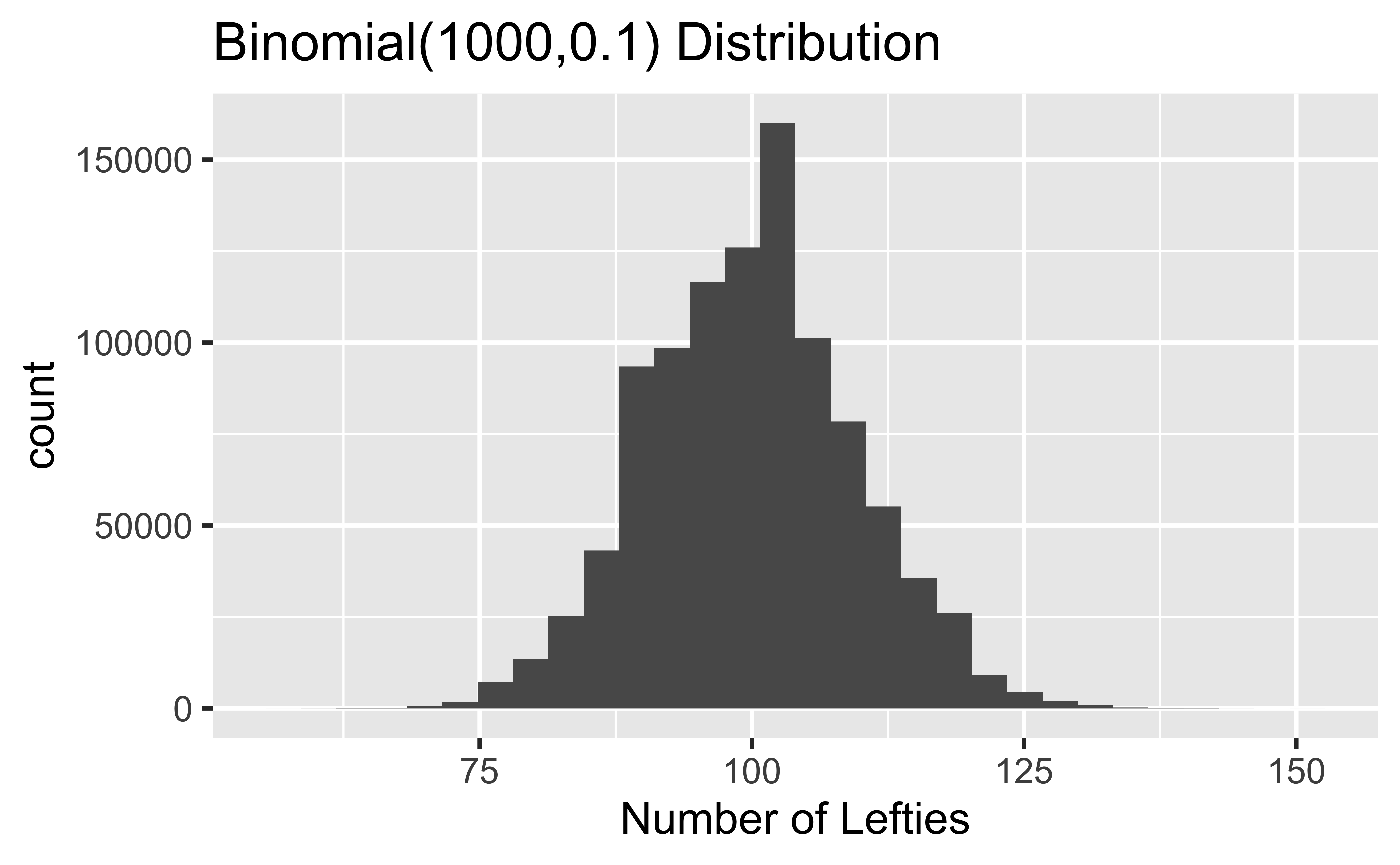
\[\begin{aligned} \begin{pmatrix} n \\ x \end{pmatrix}\pi^x(1-\pi)^{n-x} & = \frac{n!}{x!(n-x)!}\pi^x(1-\pi)^{n-x} \\ \begin{pmatrix} 3 \\ 3 \end{pmatrix}0.1^3(1-0.1)^{3-3} & = \frac{3!}{3!(3-3)!}0.1^3(1-0.1)^{3-3} \\ & \frac{3(2)(1)}{3(2)(1)1}0.1^3(0.9)^{0}=0.1^3 \\ & = 0.001. \end{aligned}\]

Distribution of lefties

Let’s use R to take a look at the distribution of the number of lefties in groups of varying size. We can actually run an experiment in R. Let’s draw a single random sample of 1000 people with probability of being left handed of 0.1. Our random variable $X$ is now the number of lefties in this big sample.

In this experiment, how many lefties do we expect to see?

A binomial random variable has expectation (mean) $n\pi$, so we expect to see somewhere around 1000(0.1)=100 lefties.

Distribution of lefties

# If I want to reproduce my random draw exactly, I have to set
# the seed.  Otherwise, I'll get a different random sample every # time
set.seed(121372) 
# in R, what we called "n" is called size
# R's "n" is the number of experiments to run
# in this case, that's the # of samples of size 1000 to simulate
rbinom(n=1,size=1000,prob=0.1)

[1] 85

In this case, we got $X=85$ lefties, pretty close to the expectation of $n\pi=1000(0.1)=100$.

You can try setting a different seed and taking another sample for comparison (or keeping the seed and running the sampling code more than once)! We expect to see differences each time, as the process is random.

Distribution of lefties

Now suppose instead of taking a single random sample, we want to run our experiment 10 times.

rbinom(n=10,size=1000,prob=0.1)

 [1] 101  93 117  95  92  82 104  96  95  91

We can see that for each of our 10 experiments, $X$ is pretty close to its expectation (population mean) of 100 lefties.

Distribution of lefties

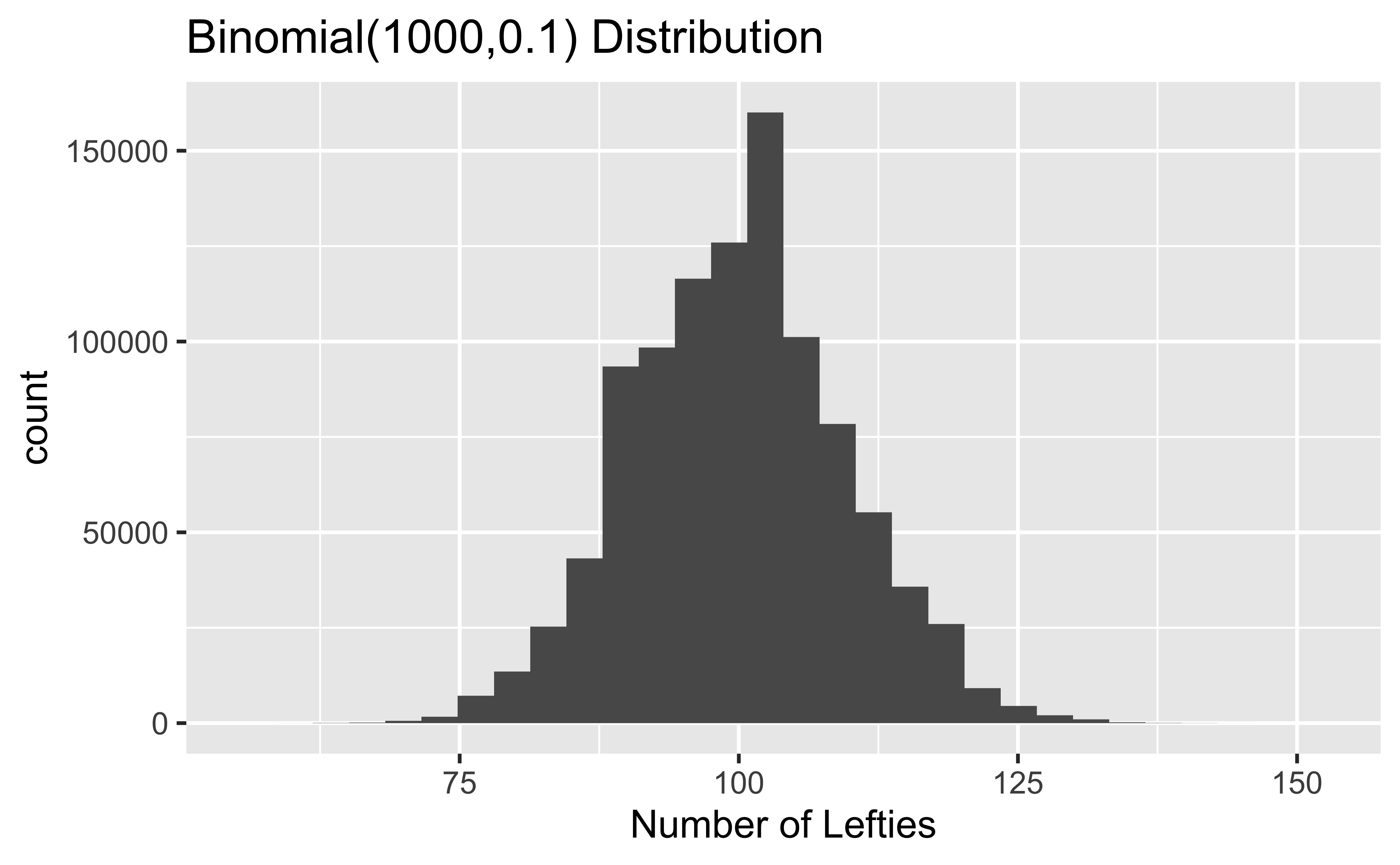
If we run the experiment a very large number of times, we can get a good estimate of the distribution, which in this case is a binomial(n=1000,0.196) distribution.

binomdata = 
  data.frame(X = rbinom(1000000, 1000, 0.1))
ggplot(binomdata, aes(x = X)) + 
  geom_histogram() +
  labs(x = "Number of Lefties",
       title = "Binomial(1000,0.1) Distribution")

New lefty study

Suppose you conduct a survey of 1000 Chinese citizens and find that 30 claim they are left-handed. If we estimate the probability of left-handedness based on the proportion who reported left-handedness in this survey, what is our estimate? Based on these data, do you think the rate of left-handedness in China is equivalent to that for the US as a whole? Why or why not?

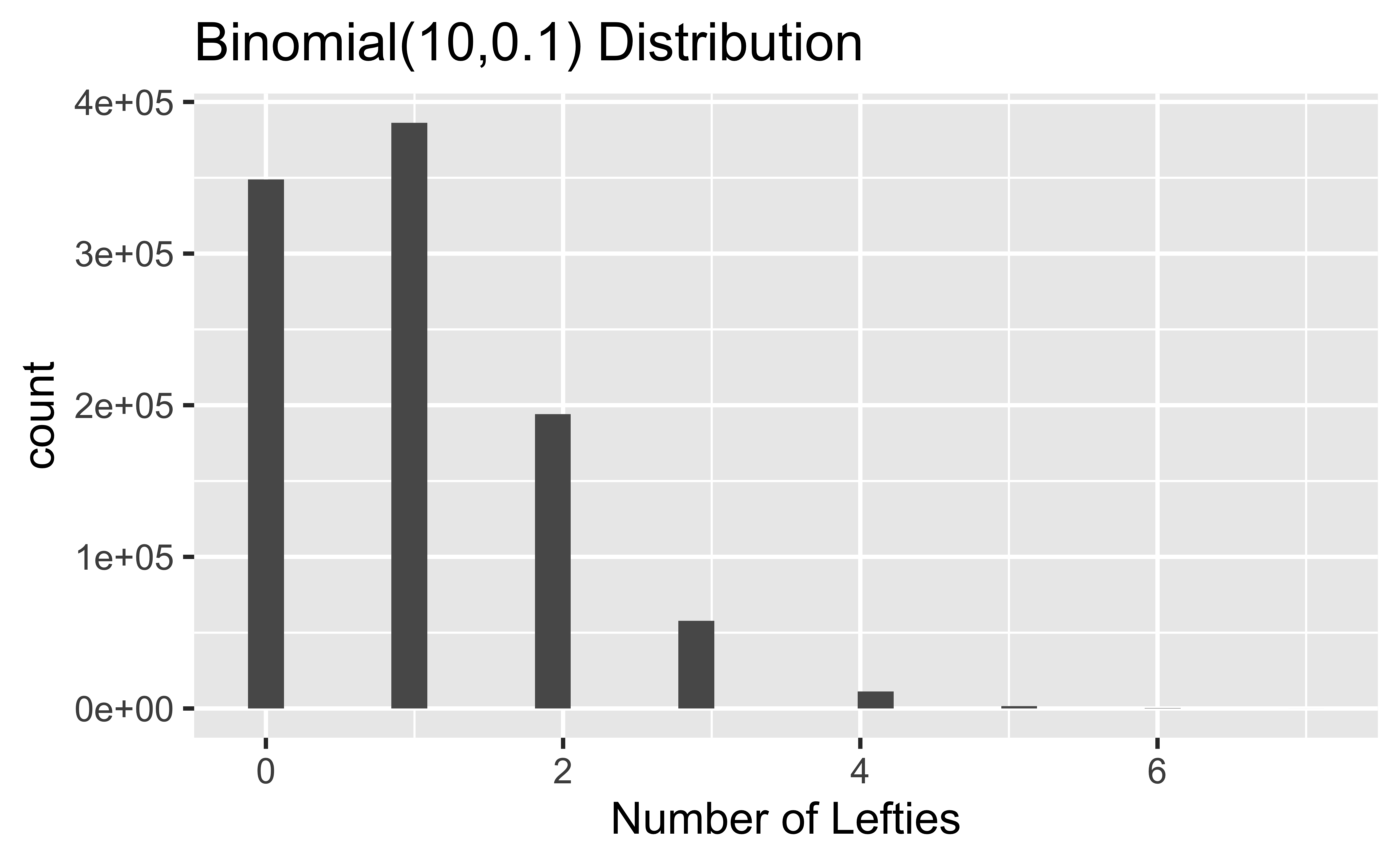
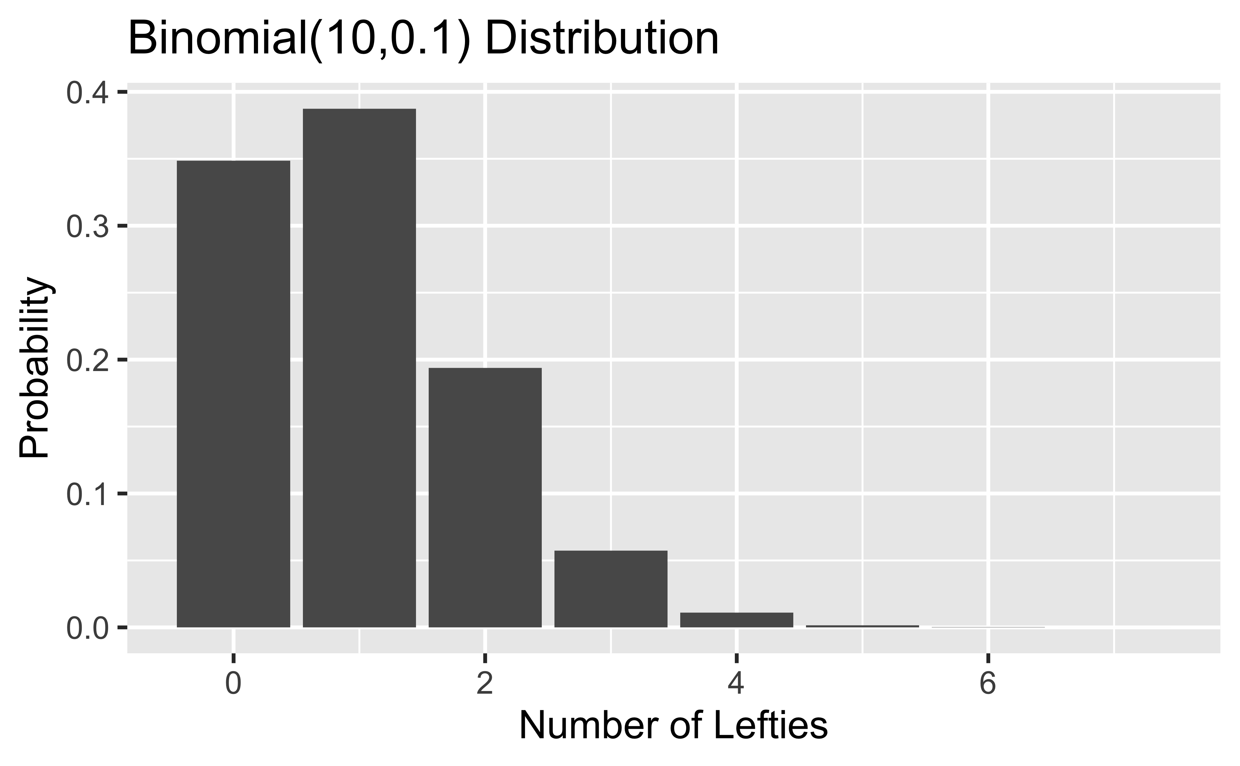
Now suppose that because of the time and money involved, you could only survey 10 Chinese citizens. The plot shows the binomial distribution with the same probability of left-handedness (10%) but with samples of $n=10$ students. (Question: why don’t the bars touch here, when they appeared to touch before?)

binomdatasmall = 
  data.frame(X = rbinom(1000000, 10, 0.1))

ggplot(binomdatasmall, aes(x = X)) + 
  geom_histogram() +
  labs(x = "Number of Lefties",
       title = "Binomial(10,0.1) Distribution")

If we survey 10 students, and they are all right-handed, what is our estimate of left-handedness from the sample?

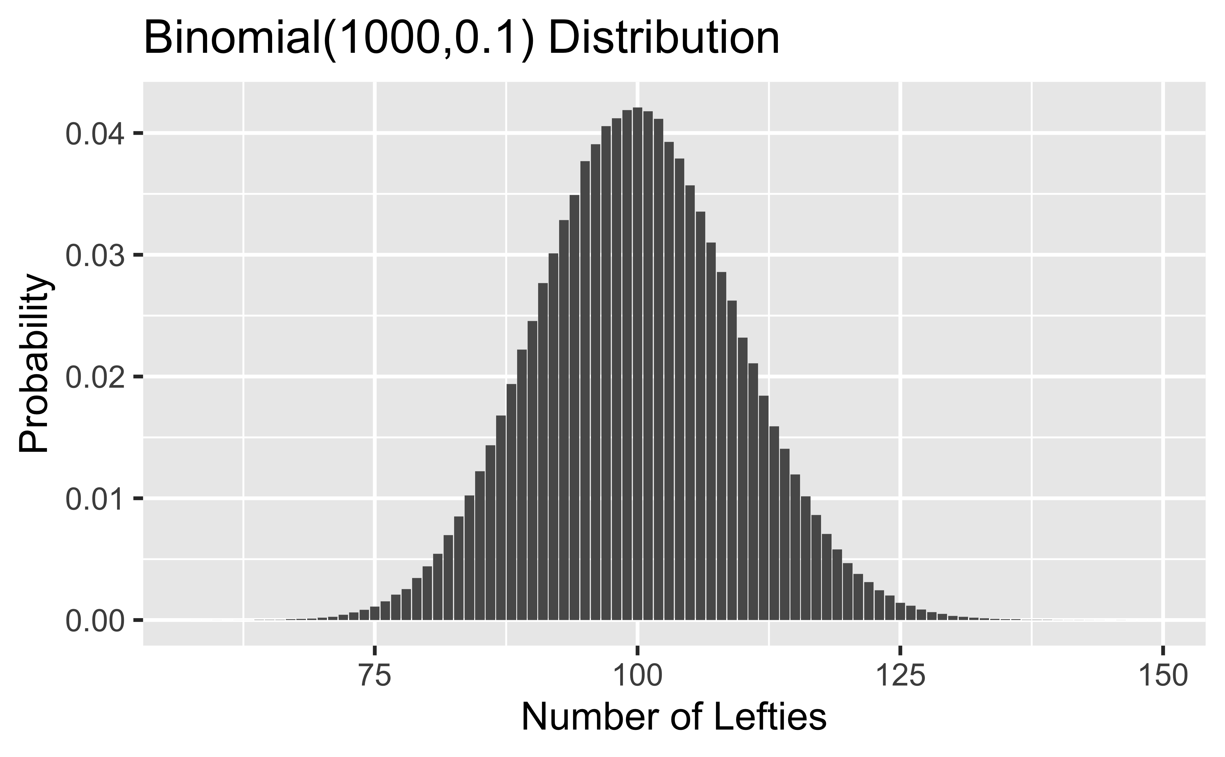
Here we compare the studies of different sizes, with the y-axis changed to a probability scale.

Why is the scale for the probabilities on the left so much smaller than that for the probabilities on the right?
Looking at the histograms, what is the most likely estimated probability of left-handedness from studies of each size?
What is the range of estimated probabilities we might expect from studies of 10 vs studies of 1000? How might this affect design of a study?

Example: Lefties in Class

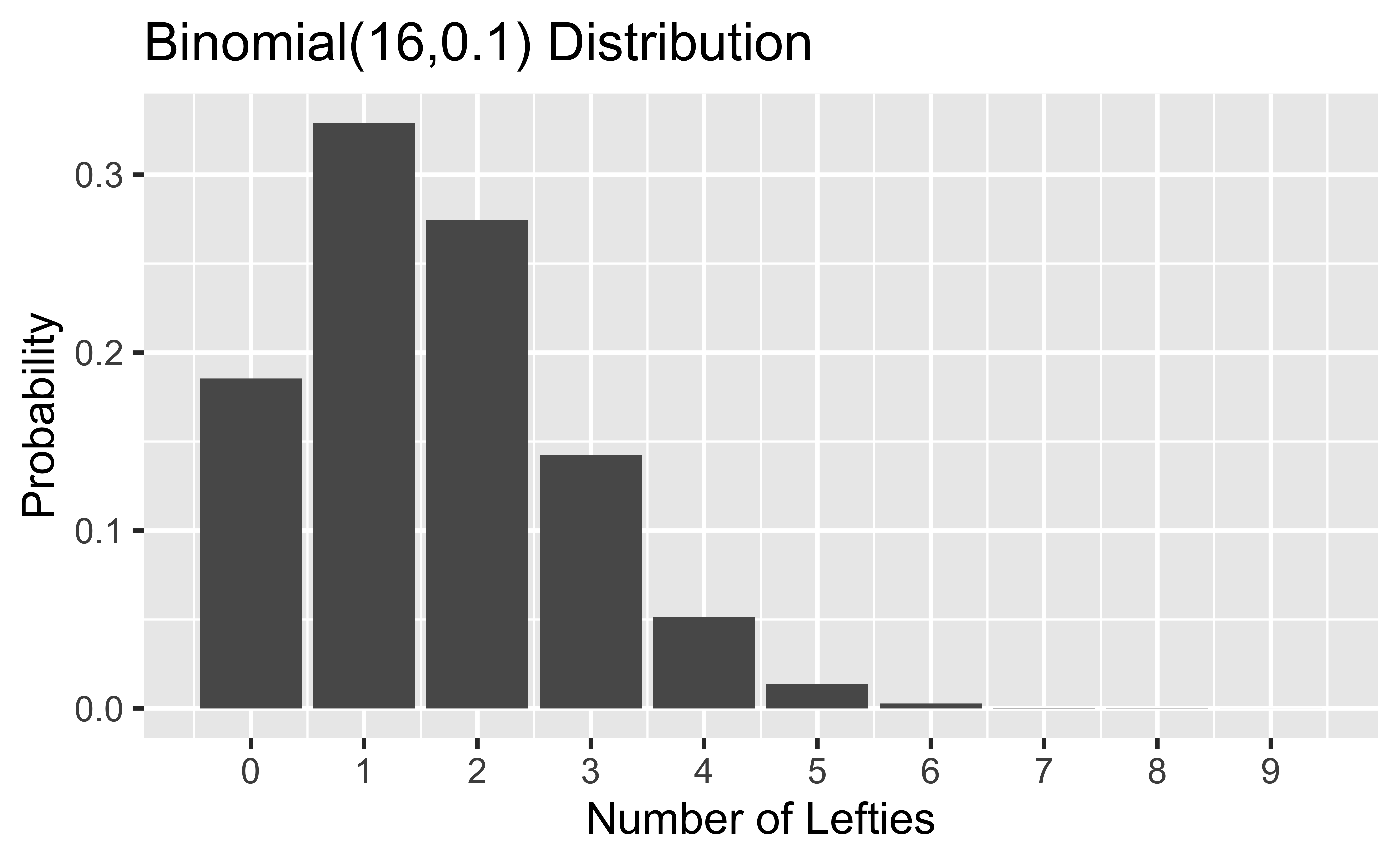
Where do we fall in the distribution? Here I’ve generated a large number of samples of size 16, assuming the 10% prevalence of left-handedness.

Example: IVF Planning

In Vitro Fertilization (IVF)

Infertility is a global health problem that is inadequately addressed worldwide. Some estimates indicate up to 2-5% of births in Western countries are through IVF.

Suppose the average success (live birth) rate of this procedure per embryo implanted is 50% (precise success rates depend on parental characteristics such as age). In the US and in many other countries, IVF is expensive and unlikely to be covered by insurance. Because of the expense (e.g., $, time, physical), parents wish to minimize the needed number of IVF treatments (i.e., maximize the success rate of a given IVF attempt).

Embryos

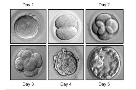
Here’s what embryos look like in the first days after conception. Note that days are counted differently in regular pregnancies vs. IVF. In a regular pregnancy, dating is done back to the first day of the last menstrual period (there is no good marker of conception). So on day 1 of a typical pregnancy, a woman is not pregnant! Ovulation is usually around day 14 of the cycle (and thus of pregnancy).

In IVF, counting starts on the day the egg is fertilized (corresponding to around day 14 of a regular pregnancy if the sperm meets the egg right away).

The Challenge

To maximize the success rate, specialists sometimes implant more than one embryo, especially if the patient is older or has had prior IVF failures.

The American Society for Reproductive Medicine states the overarching goal is to maximize the chance of one healthy singleton birth while minimizing multiple pregnancies. We want to determine the optimum number of embryos to implant so that the likelihood of having at least one baby is high, but the likelihood of having triplets, quadruplets, or higher-order births is low.

How do we address the challenge mathematically?

Let $X$ be the number of live births from a single IVF procedure that implants $n$ embryos. Here’s what we need to know.
- Probability of having at least one baby: $P(X \geq 1)$, which we want to be large
- Probability of having triplets, quadruplets, or a higher-order birth: $P(X>2)$, which we want to be small
- We assume the probability of each embryo surviving is independent of the others