Model Fitting and Interpretation: Part II

Introduction to Global Health Data Science

Amy Herring

Duke University
STA/GLHLTH 198 Fall 2026

2026-10-19

Working with the log transformed response

lHgfit <- linear_reg() %>% 
  set_engine("lm") %>%
  fit(lhairHg ~ assets_sc, data = mercury)
lHgfit %>% tidy(conf.int=TRUE)

#> # A tibble: 2 × 7
#>   term        estimate std.error statistic  p.value conf.low conf.high
#>   <chr>          <dbl>     <dbl>     <dbl>    <dbl>    <dbl>     <dbl>
#> 1 (Intercept)    0.280    0.0213      13.1 7.49e-38    0.238     0.321
#> 2 assets_sc     -0.358    0.0216     -16.5 3.90e-58   -0.400    -0.315

lHgfit %>% glance() %>% print(width = Inf)

#> # A tibble: 1 × 12
#>   r.squared adj.r.squared sigma statistic  p.value    df logLik   AIC   BIC
#>       <dbl>         <dbl> <dbl>     <dbl>    <dbl> <dbl>  <dbl> <dbl> <dbl>
#> 1     0.106         0.106  1.02      274. 3.90e-58     1 -3316. 6638. 6655.
#>   deviance df.residual  nobs
#>      <dbl>       <int> <int>
#> 1    2407.        2298  2300

Slope and intercept

\[ \widehat{\text{lhairHg}}_i = 0.280 - 0.358\,\text{assets\_sc}_i \]

• Slope: When assets are one standard deviation higher, the log hair mercury level is expected to be lower, on average, by 0.358 log ppm.
  • perhaps not a very useful statement given the scale
• Intercept: Individuals with household assets at the mean level (assets_sc=0) are expected to have hair mercury concentrations of 0.280 log ppm, on average
  • Remember assets_sc was standardized, so assets_sc=0 does not mean “no assets” but instead means “average assets” as it corresponds to an assets z-score of 0.

Slope and intercept: easy/standard case

Interpretation is a little easier without a log transformation. Suppose our outcome \(y\) is exam score, and the predictor \(x\) is hours studied, and we fit a linear model and get the following estimated line.

\[\widehat{y}_{i} = 60 + 5 \times x_{i}\]

• Slope: For each additional hour of study, the exam score is expected to be higher, on average, by 5 points.

• Intercept: Individuals who do not study are expected to have exam scores of 60 points, on average

• Note: now you can see the danger of extrapolating beyond the range of the data. We don’t expect someone who studies 20 hours to have an exam score of 160 on a 100-point scale – at some point, mastery (hopefully not futility!) is reached.

Better Interpretation in Models with Log Transformation

Working with logs

• Subtraction and logs: \(log(a) − log(b) = log(a / b)\)

• Natural logarithm: \(e^{log(x)} = x\)

• We can use these identities to “undo” the log transformation

Interpreting the slope

The slope coefficient for the log transformed model is -0.358, meaning the log mercury difference between people whose household incomes are one SD apart is predicted to be -0.358 (95% CI=(-0.400,-0.315)) log ppm.

Using this information, and properties of logs that we just reviewed, fill in the blanks in the following alternate interpretation of the slope:

For each additional SD the household assets are greater, the hair mercury concentration is expected to be ___ , on average, by a factor of ___.

For each additional increase in scaled assets, hair mercury content is expected to be ___ , on average, by a factor of ___.

\[ \log(\text{hair Hg for assets x+1}) - \log(\text{hair Hg for assets x}) = -0.358 \]

\[ \log\left(\frac{\text{hair Hg for assets x+1}}{\text{hair Hg for assets x}}\right) = -0.358 \]

\[ e^{\log\left(\frac{\text{Hg for assets x+1}}{\text{Hg for assets x}}\right)} = e^{-0.358} \]

\[ \frac{\text{Hg for assets x+1}}{\text{Hg for assets x}} \approx 0.70 \]

When assets are one standard deviation higher, the hair Hg is expected to be lower, on average, by a factor of 0.70.

You said I didn’t need a calculator!

Yup, R can do this for you!

fit <- linear_reg() %>%
  set_engine("lm") %>%
  fit(lhairHg ~ assets_sc, data = mercury)
fit %>% tidy(exponentiate=TRUE, conf.int=TRUE)

#> # A tibble: 2 × 7
#>   term        estimate std.error statistic  p.value conf.low conf.high
#>   <chr>          <dbl>     <dbl>     <dbl>    <dbl>    <dbl>     <dbl>
#> 1 (Intercept)    1.32     0.0213      13.1 7.49e-38    1.27      1.38 
#> 2 assets_sc      0.699    0.0216     -16.5 3.90e-58    0.670     0.730

When assets are one standard deviation higher, the hair Hg is expected to be lower, on average, by a factor of 0.70 (95% CI=(0.67, 0.73)).

The Geometric Mean

The geometric mean averages positive values on the log scale, then converts back:

\[ \text{Geometric mean of } y = e^{\,\text{mean}(\log y)} \]

• Our model predicts the mean of log hair mercury at a given asset score.
• Exponentiating that prediction gives the geometric mean hair mercury in ppm.
• Therefore, \(e^{-0.358}\approx 0.70\) compares two predicted geometric means: at an asset score one standard deviation higher, the geometric mean is about 70% as high, or 30% lower.

Because mercury concentrations are right-skewed, the geometric mean is generally lower than the arithmetic mean. They should not be interpreted as the same quantity, strictly speaking.

When is a geometric mean useful?

• For positive, right-skewed measurements, such as many exposure concentrations.
• When we want to describe proportional differences: “30% lower” rather than “0.89 ppm lower.”
• When a few very high values would strongly pull up the arithmetic mean.

Use the arithmetic mean when the question is about the average amount in ppm or a total across people. A geometric mean requires positive values.

From a ratio to a percentage

We found that a one-standard-deviation increase in assets multiplies the predicted geometric mean hair mercury concentration by

\[e^{-0.358} \approx 0.70.\]

• 0.70 times as high means 70% as high.
• \(100\%(1-0.70)=30\%\) lower.

Interpretation: People whose household asset score is one standard deviation higher have a predicted geometric mean hair mercury concentration about 30% lower.

A reusable rule

If we fit a model for \(\log(y)\) and the slope is \(\widehat\beta_1\):

\[ \text{Multiplier for a one-unit increase in }x = e^{\widehat\beta_1} \]

\[ \text{Percentage change} = \left(e^{\widehat\beta_1}-1\right)\times100\%. \]

• Negative result: a percentage decrease.
• Positive result: a percentage increase.
• Use the exponential, not \(100\widehat\beta_1\%\), for the exact percentage change.

Let R do the conversion

Code

tidy(lHgfit$fit, conf.int = TRUE) %>%
  filter(term == "assets_sc") %>%
  mutate(
    multiplier = exp(estimate),
    percent_change = 100 * (exp(estimate) - 1),
    ci_low = 100 * (exp(conf.low) - 1),
    ci_high = 100 * (exp(conf.high) - 1)
  ) %>%
  select(term, multiplier, percent_change, ci_low, ci_high) %>%
  mutate(across(where(is.numeric), ~round(.x, 1)))

Output

#> # A tibble: 1 × 5
#>   term      multiplier percent_change ci_low ci_high
#>   <chr>          <dbl>          <dbl>  <dbl>   <dbl>
#> 1 assets_sc        0.7          -30.1    -33     -27

The estimate is approximately −30.1%. The 95% confidence interval is approximately −33.0% to −27.0%.

Interpreting the confidence interval

For a one-standard-deviation difference in household assets:

\[ 95\%\ \text{CI for the multiplier:}\quad \left(e^{-0.400},\ e^{-0.315}\right) \approx (0.67,\ 0.73). \]

• The predicted geometric mean hair mercury concentration is estimated to be 27% to 33% lower at the higher asset score.
• The interval excludes a multiplier of 1, equivalent to excluding a percentage change of 0%.

What about the intercept?

\[ \widehat{\log(\text{hair Hg})} = 0.280 - 0.358\,\text{assets\_sc} \]

• At assets_sc = 0 (average assets): \(e^{0.280}\approx\mathbf{1.32}\) ppm.
• At assets_sc = 1: \(e^{0.280-0.358}\approx\mathbf{0.92}\) ppm.
• Compare: \(0.92/1.32\approx 0.70\), or about 30% lower.

These are predictions for the geometric mean, not the arithmetic mean mercury concentration in ppm.

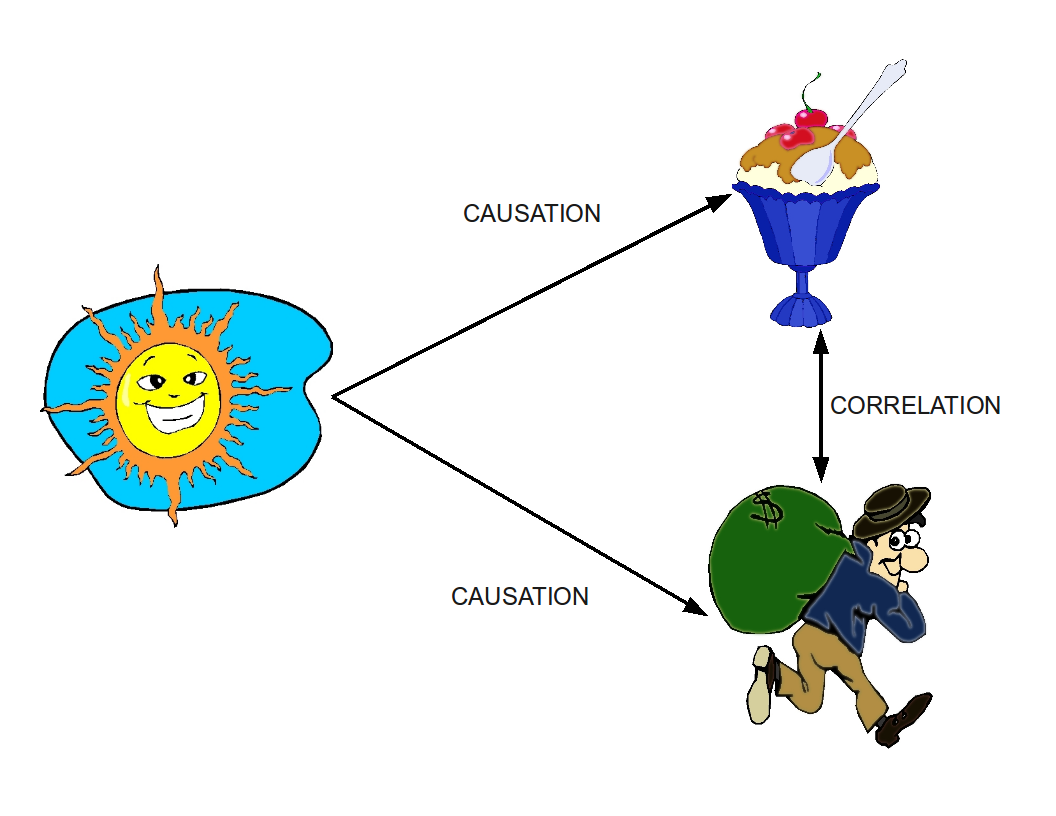
Correlation does not imply causation

Remember this when interpreting model coefficients!

Illustration: Rcragun, Wikimedia Commons, CC BY 3.0

Source: xkcd, “Correlation”

Estimation Details

Linear model with a single predictor

• We’re interested in \(\beta_0\) (population parameter for the intercept) and \(\beta_1\) (population parameter for the slope) in the following model:

\[y_{i} = \beta_0 + \beta_1~x_{i}+\varepsilon_i\]

where \(\varepsilon\) represents random error around our mean

• Tough luck, you can’t have them…

• So we use sample statistics to estimate them, using the notation \(b\) or \(\widehat{\beta}\) to distinguish our estimates from the true parameters \(\beta\)

\(\widehat{y}_{i} = b_0 + b_1~x_{i}\) or \(\widehat{y}_i = \widehat{\beta}_0 + \widehat{\beta}_1~x_i\)

Least squares regression

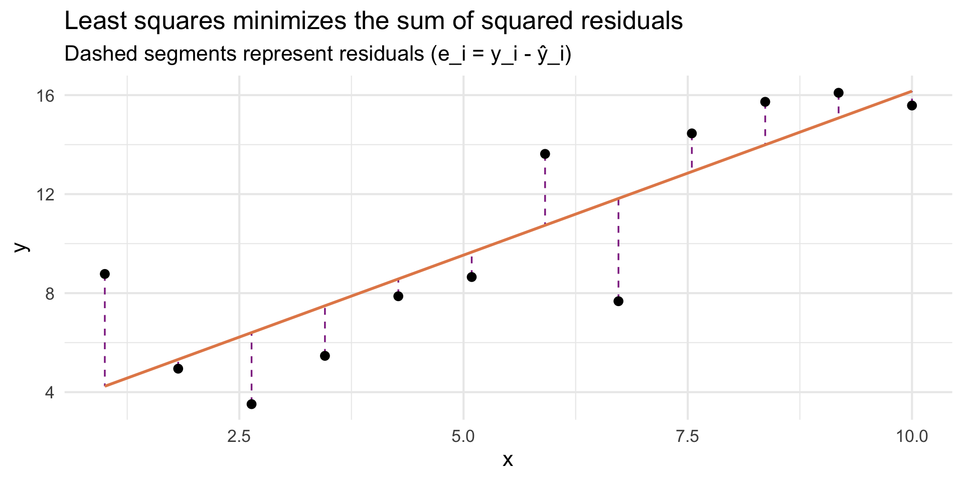
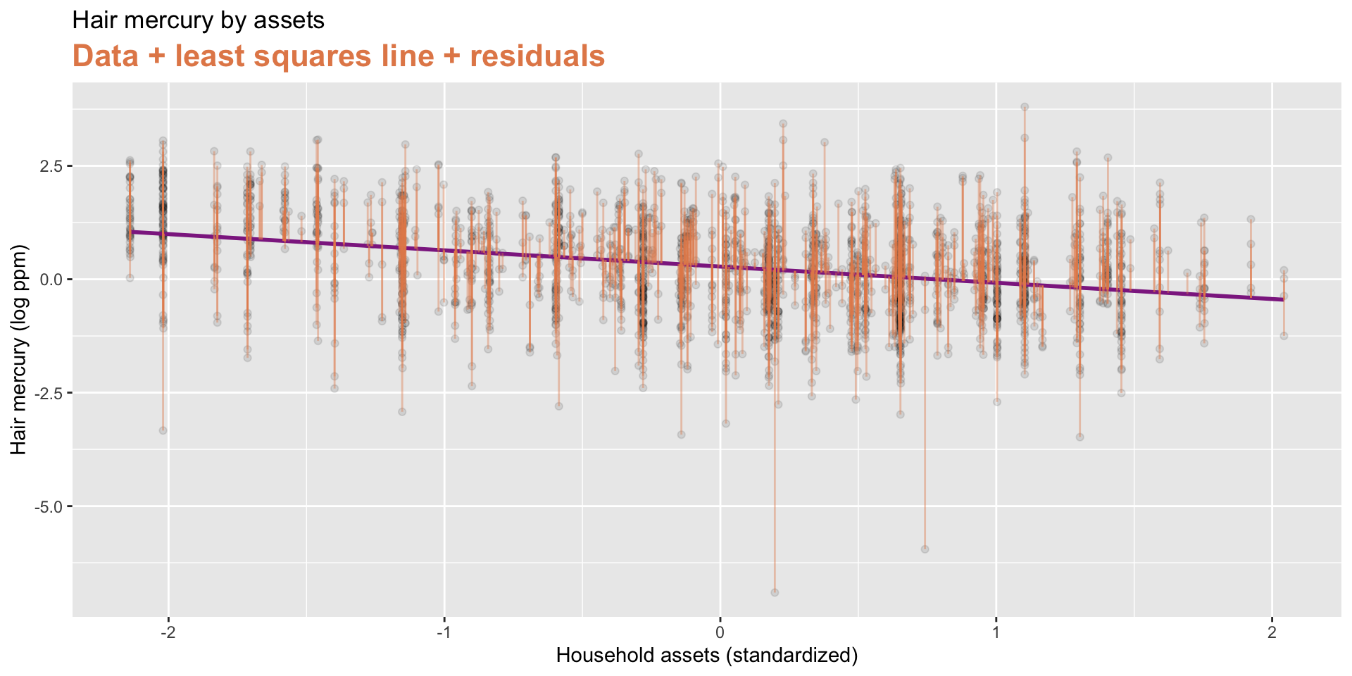
• The regression line minimizes the sum of squared residuals (the residuals are estimates of the error \(\varepsilon_i\)).

• If \(e_i = y_i - \hat{y}_i\), then, the regression line minimizes \(\sum_{i = 1}^n e_i^2\).

• Why do we square the residuals?

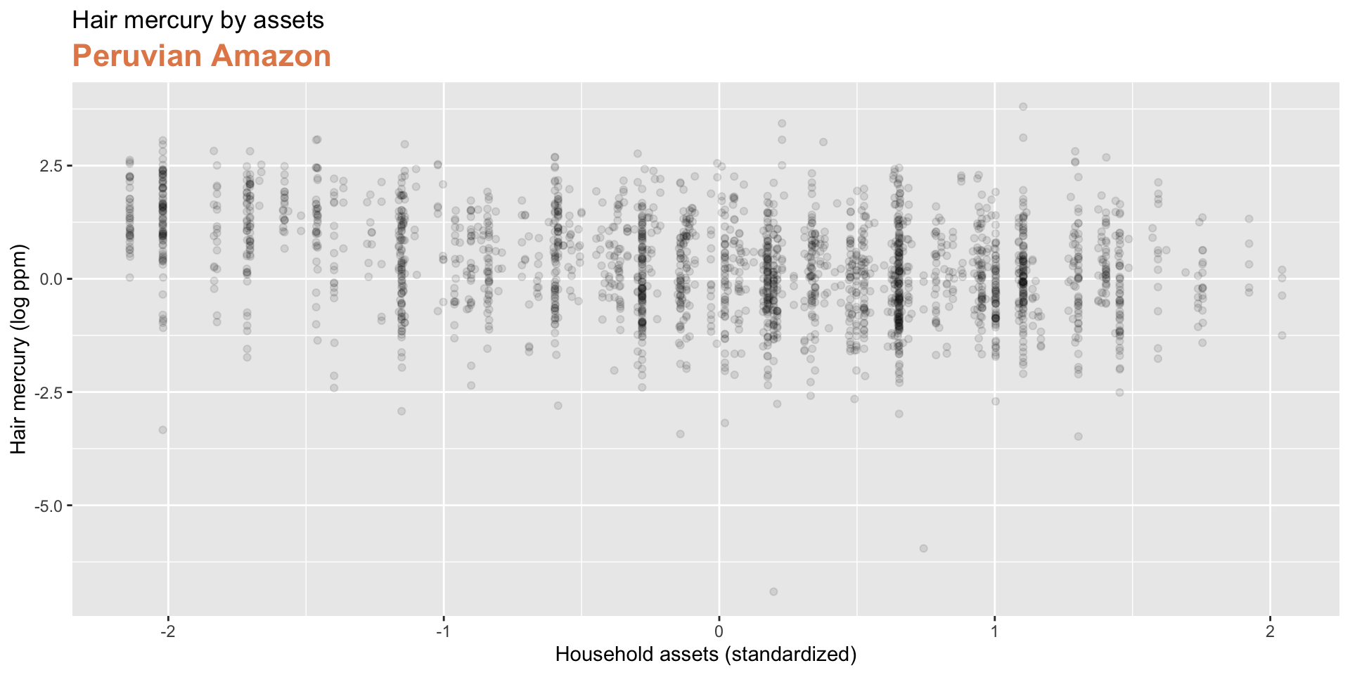
Visualizing residuals

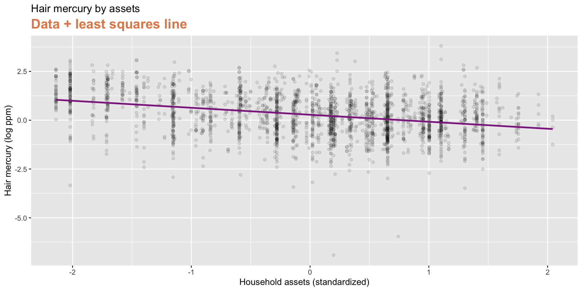
Visualizing residuals (cont.)

Visualizing residuals (cont.)

How well does the model fit? \(R^2\)

The coefficient of determination, \(R^2\), measures the proportion of variation in the response \(y\) that is explained by the regression model.

\[ R^2 = 1 - \frac{\sum_{i=1}^n (y_i-\widehat{y}_i)^2} {\sum_{i=1}^n (y_i-\bar{y})^2} \]

• \(\sum (y_i-\widehat{y}_i)^2\): variation not explained by the model
• \(\sum (y_i-\bar{y})^2\): total variation in \(y\)

\(R^2\) ranges from 0 to 1.

• \(R^2 = 0\): the model explains none of the variation in \(y\)
• \(R^2 = 1\): the model explains all of the variation in \(y\)

For simple linear regression with one predictor:

\[ R^2 = r^2 \]

We can get \(R^2\) from the glance function.

fit <- linear_reg() %>%
  set_engine("lm") %>%
  fit(lhairHg ~ assets_sc, data = mercury)
fit %>% glance() %>% print(width = Inf)

#> # A tibble: 1 × 12
#>   r.squared adj.r.squared sigma statistic  p.value    df logLik   AIC   BIC
#>       <dbl>         <dbl> <dbl>     <dbl>    <dbl> <dbl>  <dbl> <dbl> <dbl>
#> 1     0.106         0.106  1.02      274. 3.90e-58     1 -3316. 6638. 6655.
#>   deviance df.residual  nobs
#>      <dbl>       <int> <int>
#> 1    2407.        2298  2300

While \(R^2=0.106\) may seem quite low (the corresponding estimated correlation between \(x\) and \(y\) is \(\sqrt{0.106}=0.33\)), it’s actually not too alarming given that we have observational data from humans with highly variable activities and exposures.

Properties of least squares regression

• The regression line goes through the center of mass point, the coordinates corresponding to average \(x\) and average \(y\), \((\bar{x}, \bar{y})\):
  \[\bar{y} = \hat{\beta}_0 + \hat{\beta}_1 \bar{x} ~ \rightarrow ~ \hat{\beta}_0 = \bar{y} - \hat{\beta}_1 \bar{x}\]

• The slope has the same sign as the correlation coefficient: \(\hat{\beta}_1 = r \frac{s_y}{s_x}\)
  • \(s_x\) is the standard deviation of the explanatory variable \(x\), and \(s_y\) is the standard deviation of the response variable \(y\)
  • If \(y\) varies a lot more than \(x\) does (large \(s_y\) relative to \(s_x\)), the slope will be steeper for the same correlation — a small change in \(x\) corresponds to a much bigger typical change in \(y\)
  • In our example, \(s_x\) is the standard deviation of assets_sc (which is 1, since it was standardized), and \(s_y\) is the standard deviation of lhairHg

• The sum of the residuals is zero: \(\sum_{i = 1}^n e_i = 0\)

• The residuals and \(x\) values are uncorrelated

Model checking

“Linear” models

• We’re fitting a “linear” model, which assumes a linear relationship between our explanatory and response variables.
• But how do we assess this?
• We saw residual plots earlier – let’s dive in with more detail now!

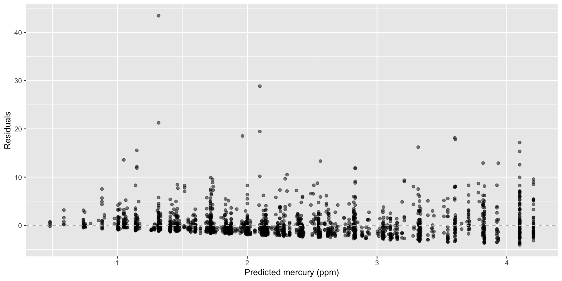
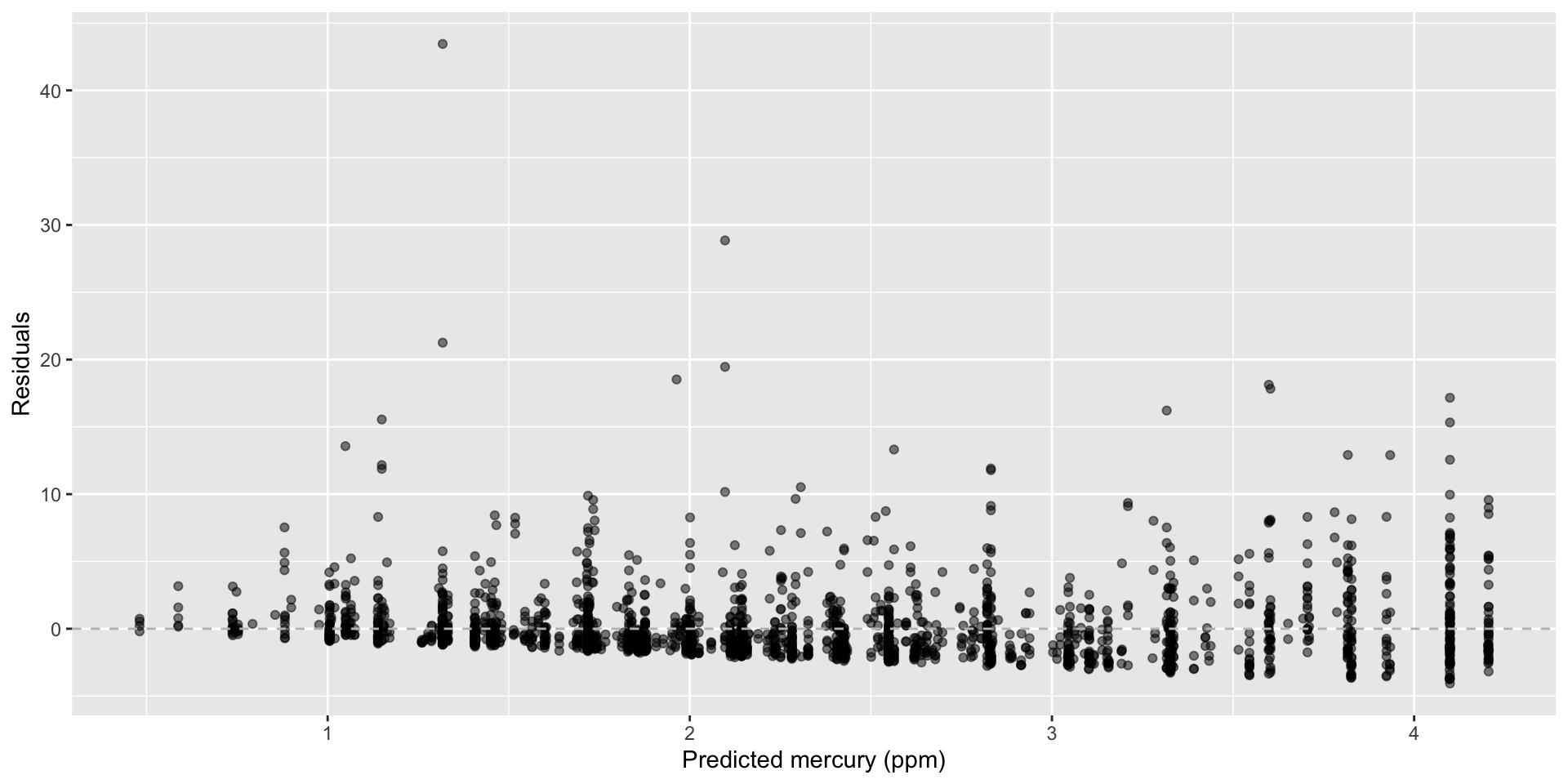
Graphical diagnostic: residuals plot (ppm units)

• Plot
• Code
• Augment

hg_asset_fit <- linear_reg() %>%
  set_engine("lm") %>%
  fit(hairHg ~ assets_sc, data = mercury)
hg_asset_fit_aug <- augment(hg_asset_fit$fit)
ggplot(hg_asset_fit_aug, mapping = aes(x = .fitted, y = .resid)) +
  geom_point(alpha = 0.5) +
  geom_hline(yintercept = 0, color = "gray", lty = "dashed") +
  labs(x = "Predicted mercury (ppm)", y = "Residuals")

hg_asset_fit_aug

#> # A tibble: 2,300 × 9
#>    .rownames hairHg assets_sc[,1] .fitted .resid     .hat .sigma    .cooksd
#>    <chr>      <dbl>         <dbl>   <dbl>  <dbl>    <dbl>  <dbl>      <dbl>
#>  1 1          1.97         -0.837    3.05 -1.08  0.000750   2.77 0.0000571 
#>  2 3          1.10          0.197    2.12 -1.03  0.000452   2.77 0.0000312 
#>  3 11         5.34         -0.280    2.55  2.79  0.000471   2.77 0.000239  
#>  4 13         1.57         -0.280    2.55 -0.981 0.000471   2.77 0.0000296 
#>  5 14         2.02         -0.280    2.55 -0.528 0.000471   2.77 0.00000855
#>  6 15         0.599        -0.280    2.55 -1.95  0.000471   2.77 0.000117  
#>  7 16         0.883         0.826    1.56 -0.682 0.000737   2.77 0.0000224 
#>  8 17         0.902         0.826    1.56 -0.663 0.000737   2.77 0.0000211 
#>  9 19         1.42         -1.27     3.43 -2.01  0.00116    2.77 0.000308  
#> 10 21         1.05         -1.27     3.43 -2.39  0.00116    2.77 0.000433  
#> # ℹ 2,290 more rows
#> # ℹ 1 more variable: .std.resid <dbl>

More on augment()

glimpse(hg_asset_fit_aug)

#> Rows: 2,300
#> Columns: 9
#> $ .rownames  <chr> "1", "3", "11", "13", "14", "15", "16", "17", "19", "21", "…
#> $ hairHg     <dbl> 1.9652, 1.0951, 5.3366, 1.5683, 2.0218, 0.5993, 0.8829, 0.9…
#> $ assets_sc  <dbl[,1]> <matrix[26 x 1]>
#> $ .fitted    <dbl> 3.045165, 2.124332, 2.549503, 2.549503, 2.549503, 2.549…
#> $ .resid     <dbl> -1.0799648, -1.0292319, 2.7870974, -0.9812028, -0.5277029, …
#> $ .hat       <dbl> 0.0007495801, 0.0004516563, 0.0004705556, 0.0004705556, 0.0…
#> $ .sigma     <dbl> 2.769771, 2.769779, 2.769252, 2.769787, 2.769841, 2.769564,…
#> $ .cooksd    <dbl> 5.708620e-05, 3.122263e-05, 2.385430e-04, 2.956514e-05, 8.5…
#> $ .std.resid <dbl> -0.3901294, -0.3717471, 1.0066782, -0.3544029, -0.1906022, …

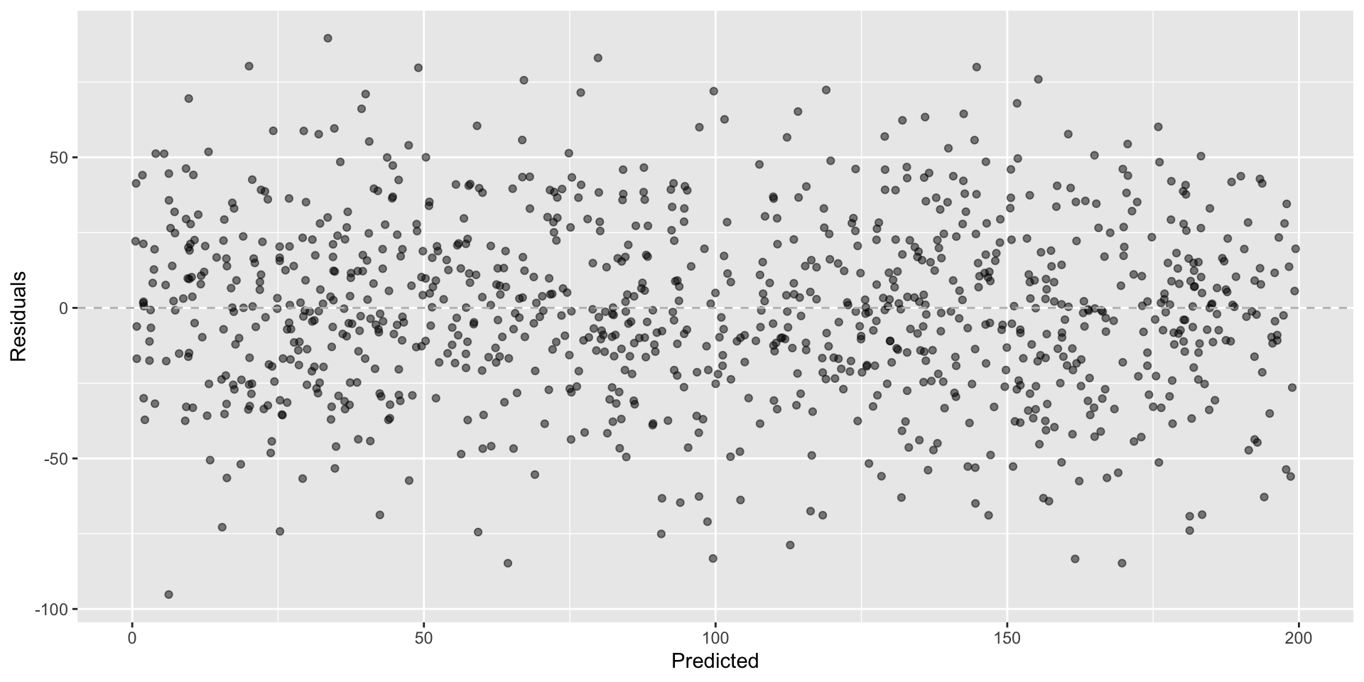
Looking for…

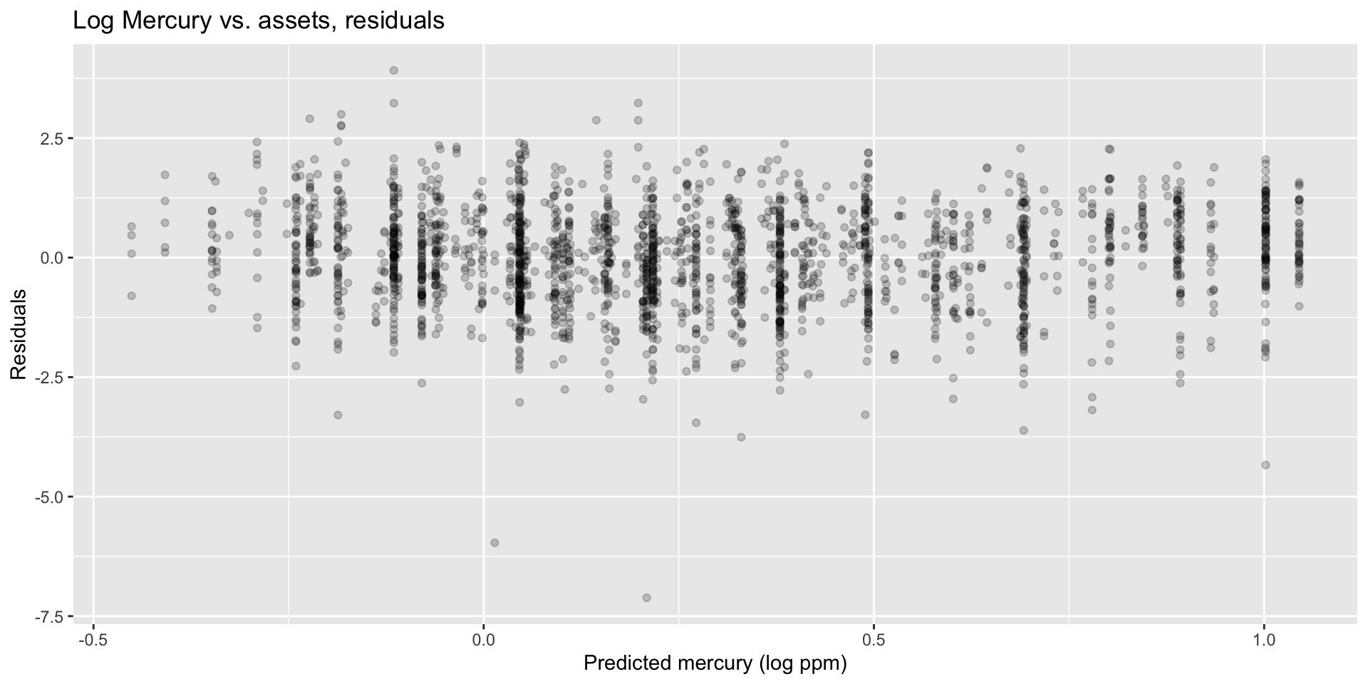
• Residuals distributed randomly around 0
• With no visible pattern along the x or y axes

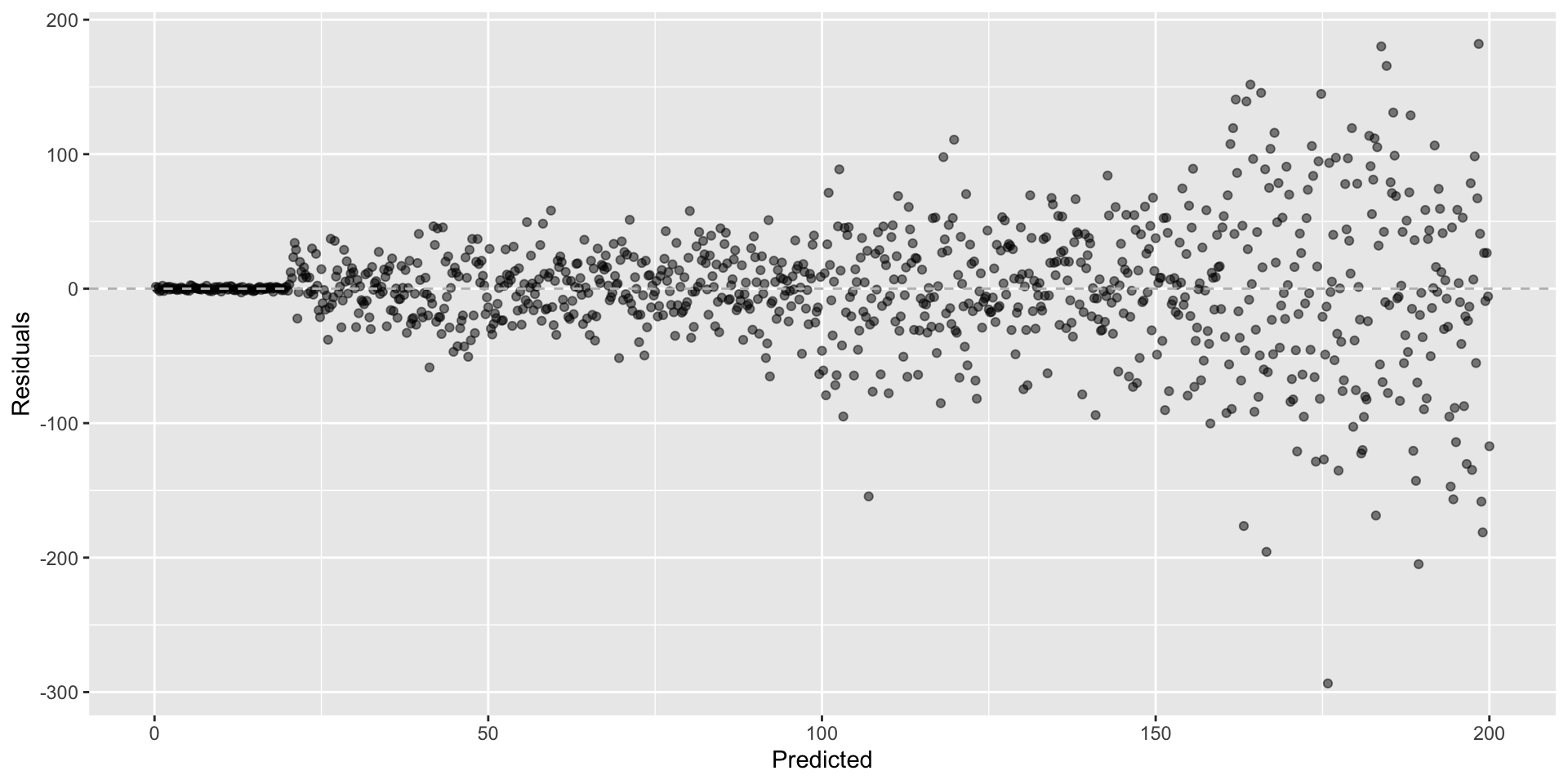
Not hoping for…

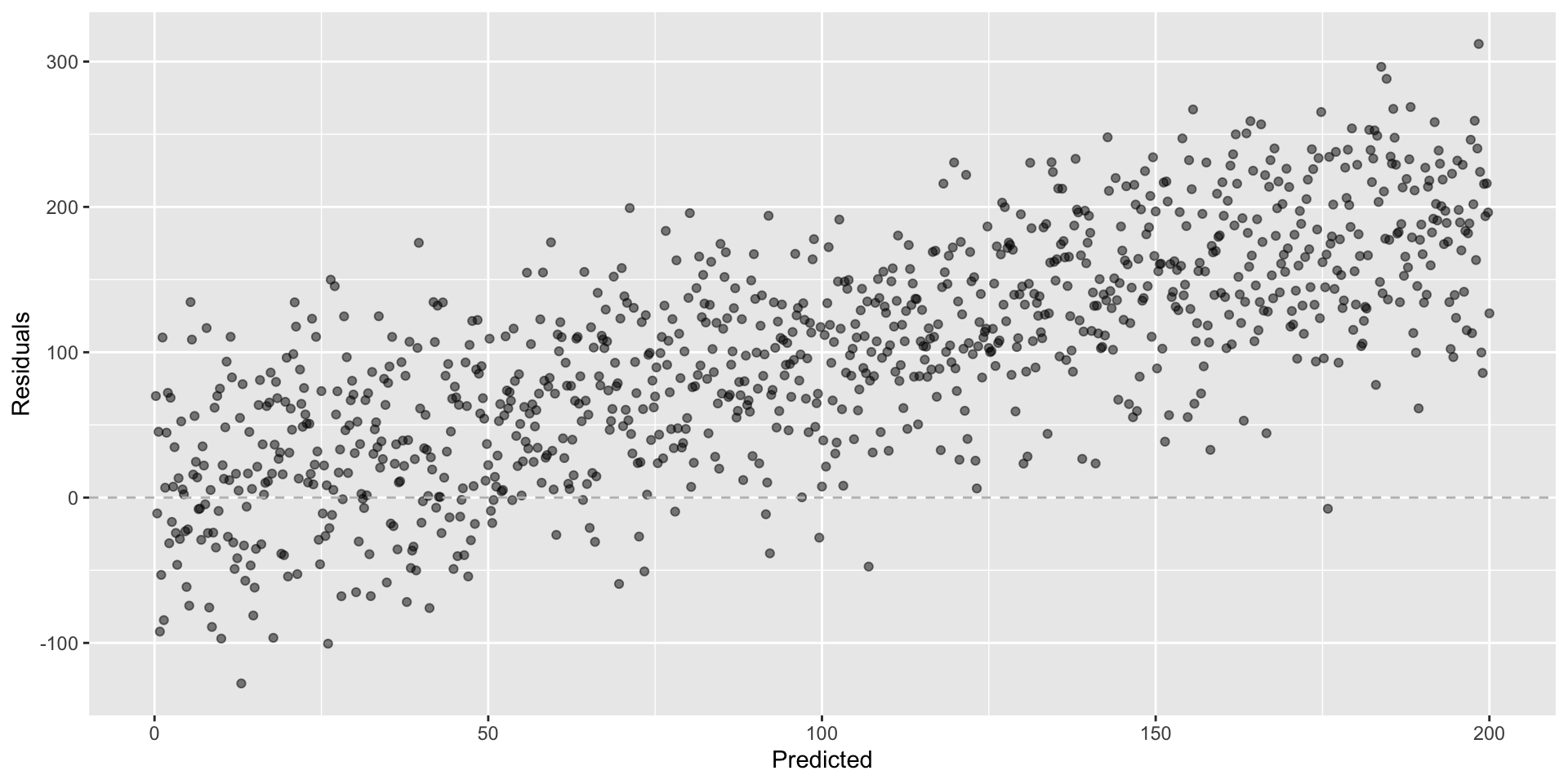
Fan shapes

(Evidence of non-constant variance in residuals across the range of predicted values)

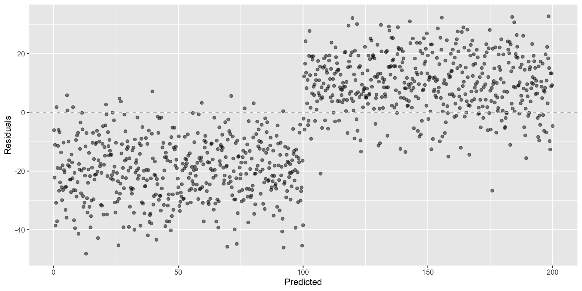
Not looking for…

Groups of patterns

(Evidence of a missing predictor)

Not looking for…

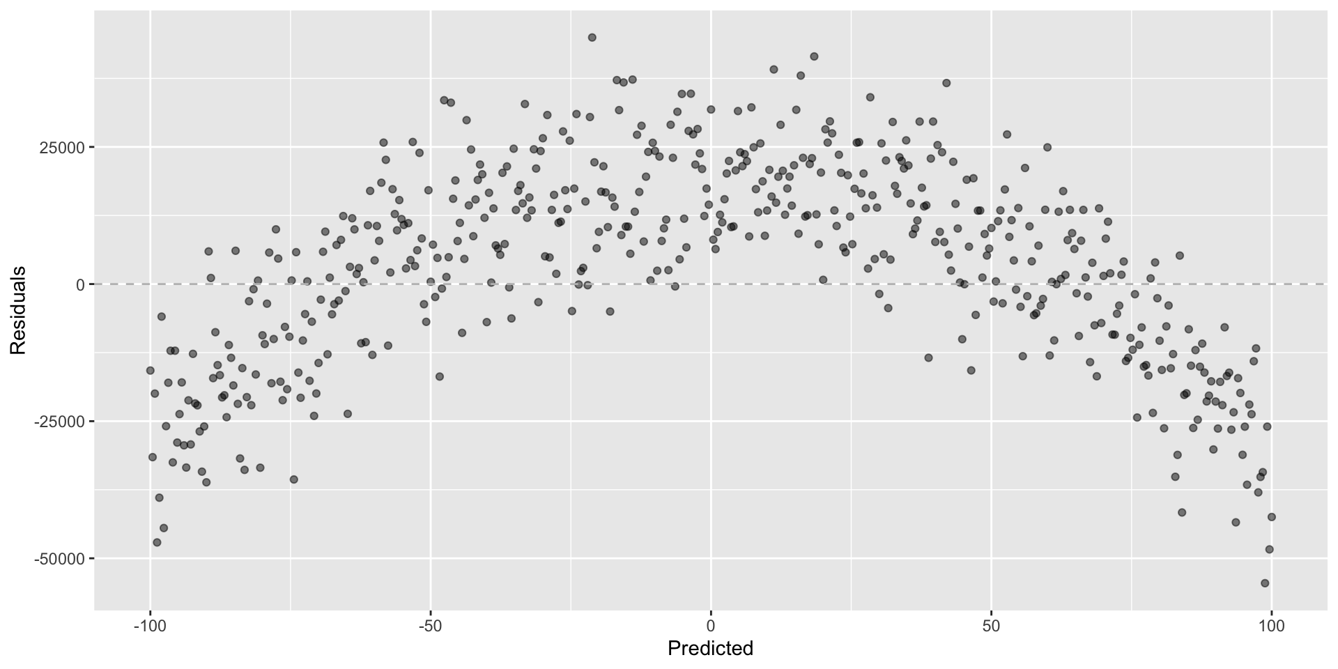
Other non-random structure

Not looking for…

Any patterns!

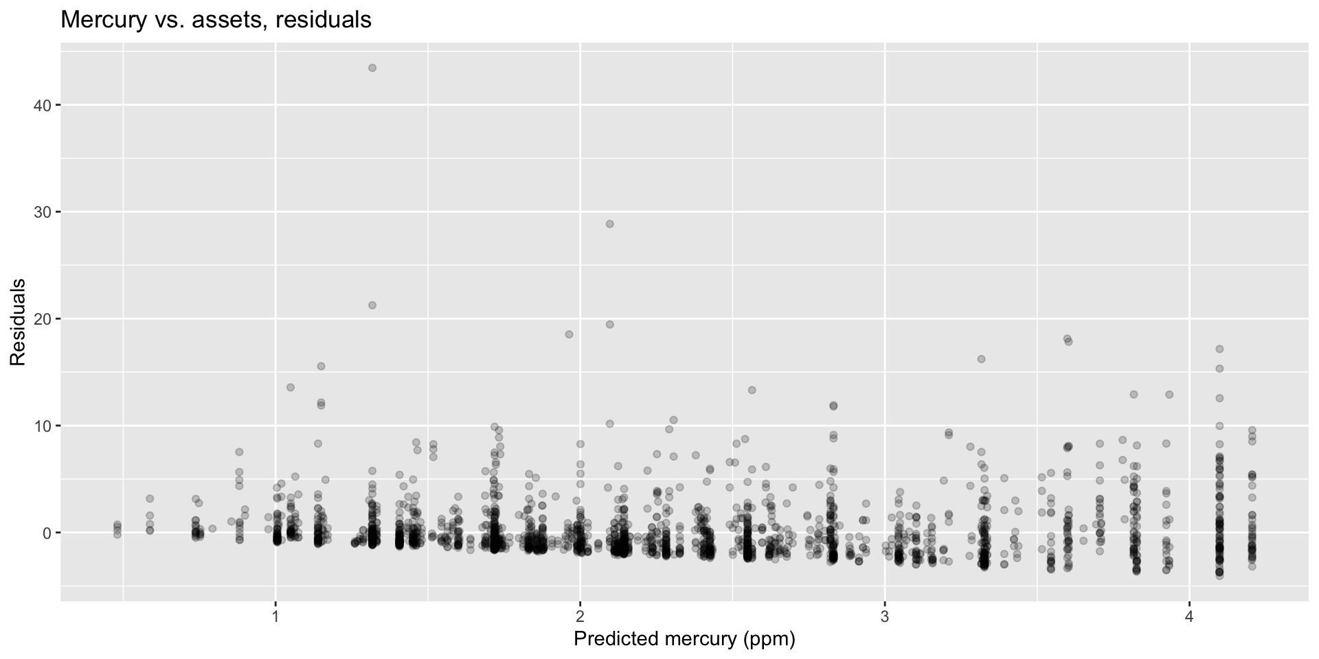
What patterns does the residual plot reveal that should make us question whether a linear model is a good fit for modeling the relationship between mercury (ppm) and assets?

Exploring linearity

Data: Mercury

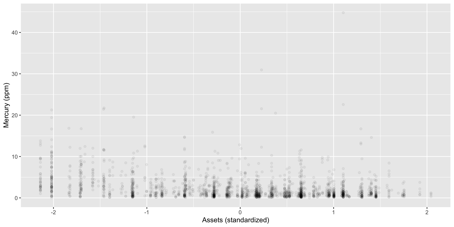
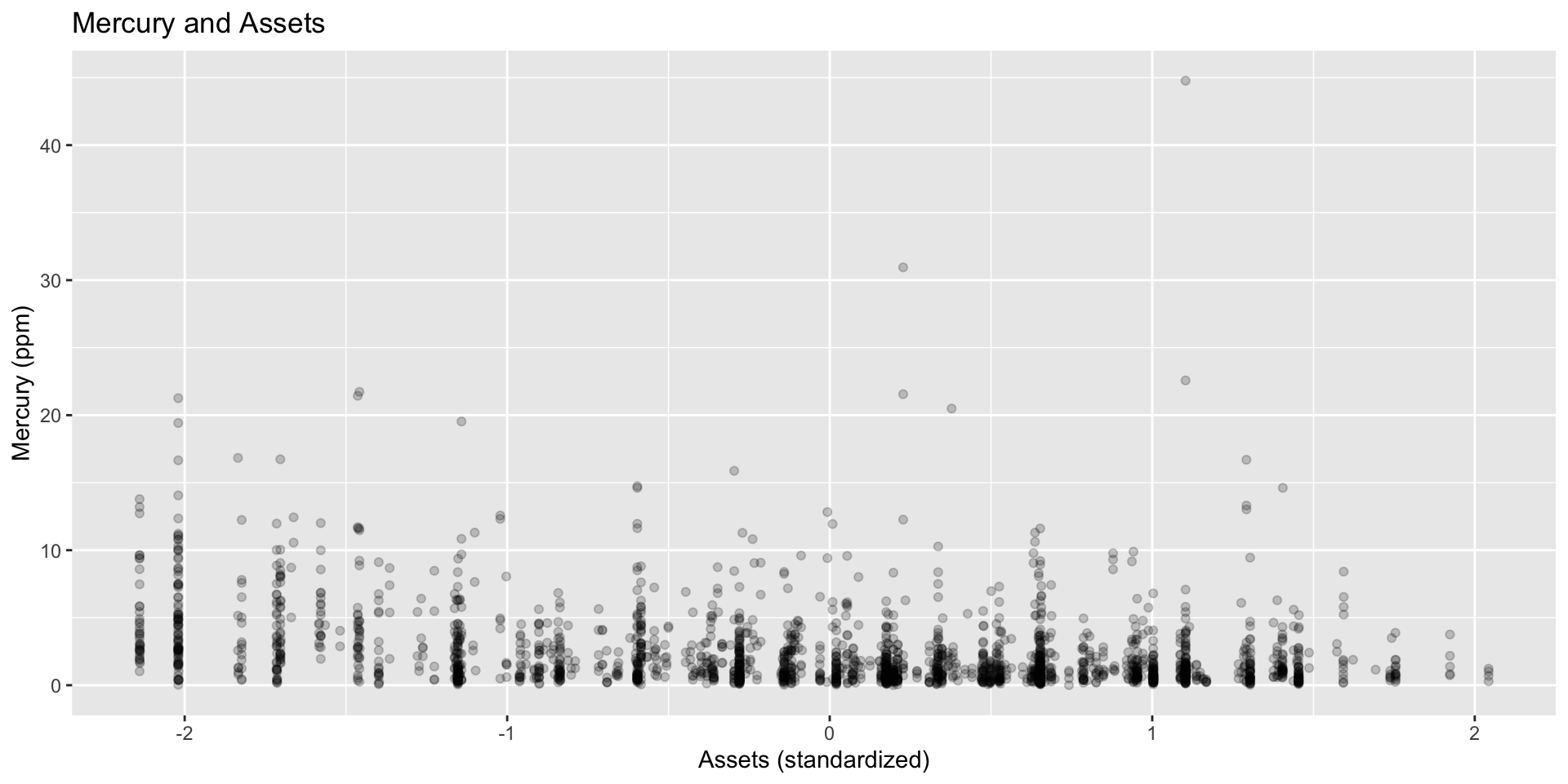
Mercury vs. assets

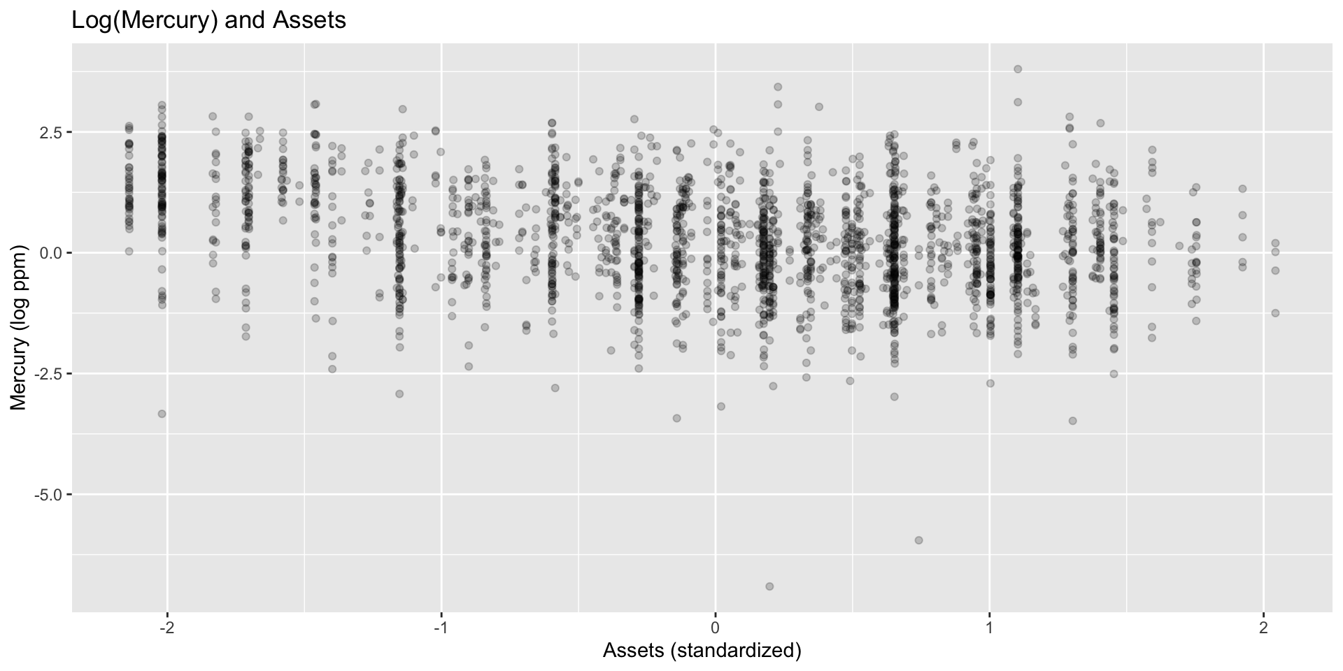
Mercury vs assets

Which plot shows a more linear relationship?

Mercury and Assets, residuals

Which plot shows a residuals that are uncorrelated with predicted values from the model? Also, what is the unit of the residuals?

Transforming the data

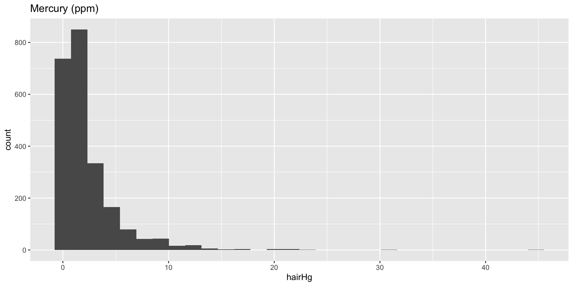
• We saw that hairHg has a right-skewed distribution, and the residuals of that model don’t look great.
• In these situations a transformation applied to the response variable may be useful.
• In order to decide which transformation to use, we should examine the distribution of the response variable.
• The extremely right skewed distribution suggests that a log transformation may be useful.
  • log = natural log, \(ln\)
  • Default base of the log function in R is the natural log:
    log(x, base = exp(1))

Transformations

• Non-constant variance is one of the most common model violations, however it is usually fixable by transforming the response (y) variable.
• The most common transformation when the response variable is right skewed is the log transform: \(log(y)\), especially useful when the response variable is (extremely) right skewed.
• This transformation is also useful for variance stabilization.
• When using a log transformation on the response variable the interpretation of the slope changes: “For each unit increase in x, y is expected on average to be higher/lower by a factor of \(e^{\hat{\beta}_1}\).”
• When the response is log-transformed, a one-unit increase in \(x\) multiplies the predicted geometric mean of \(y\) by \(e^{\hat{\beta}_1}\). This corresponds to a percentage change of \(100(e^{\hat{\beta}_1}-1)\%\); a negative result means a decrease.
• Another useful transformation is the square root: \(\sqrt{y}\), especially useful when the response variable is a count.

Transform, or learn more?

• Data transformations may also be useful when the relationship is non-linear
• However in those cases a polynomial regression may be more appropriate
  • This is beyond the scope of this course, but you’re welcomed to try it on your own, and I’d be happy to provide further guidance!

Aside: when \(y = 0\)

In some cases the value of the response variable might be 0, and

log(0)

#> [1] -Inf

The trick is to add a very small number to the value of the response variable for these cases so that the log function can still be applied:

log(0 + 0.00001)

#> [1] -11.51293

If there are a lot of 0 values for \(y\), this trick is not such a good idea, and you may need to take an alternative approach (e.g., a zero-inflated model).

Homework (Practice)

IMS Chapter 7

• Problem 7
• Problem 8
• Problem 12
• Problem 22
• Problem 23