Multiple Regression and Interaction
Introduction to Global Health Data Science
Amy Herring
Duke University
STA/GLHLTH 198 Fall 2026
2026-10-26
The linear model with multiple predictors
Multiple explanatory variables
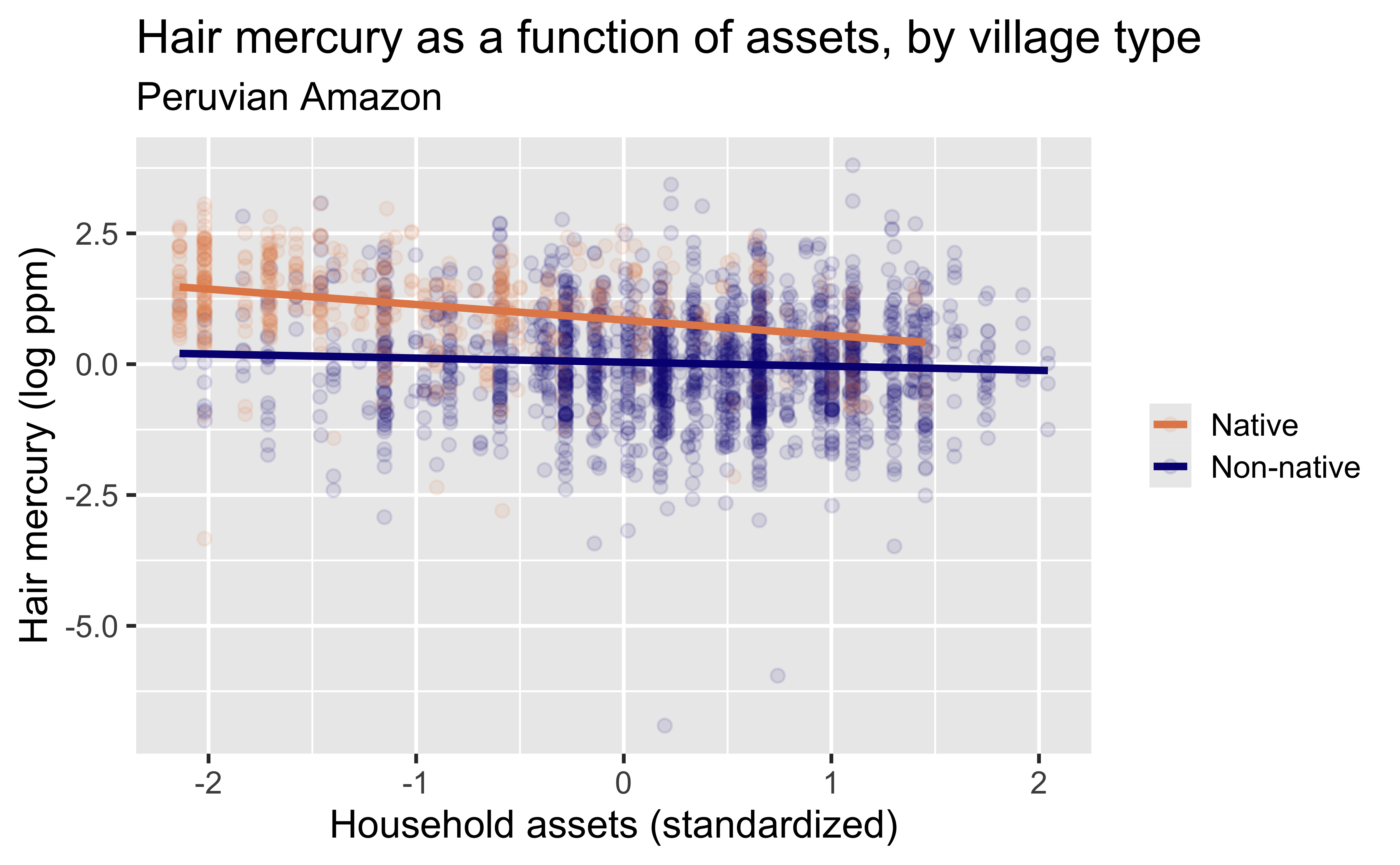
We previously explored how the relationship between assets and mercury in hair depended on whether a person lives in a native community.
How, if at all, does the relationship between hair mercury and household assets of individuals vary by whether or not they live in a town classified as native?
This is an example of an interaction effect – the relationship between assets and mercury depends on the value of a third variable, community type.
ggplot(data = mercury, aes(x = assets_sc, y = lhairHg, color = native_cat)) +
  geom_point(alpha = 0.1) +
  geom_smooth(method = "lm", se = FALSE) +
  labs(
    title = "Hair mercury as a function of assets, by village type",
    subtitle = "Peruvian Amazon",
    x = "Household assets (standardized)",
    y = "Hair mercury (log ppm)",
    color = NULL
  ) +
  scale_color_manual(values = c("#E48957", "#071381"))
Multiple explanatory variables
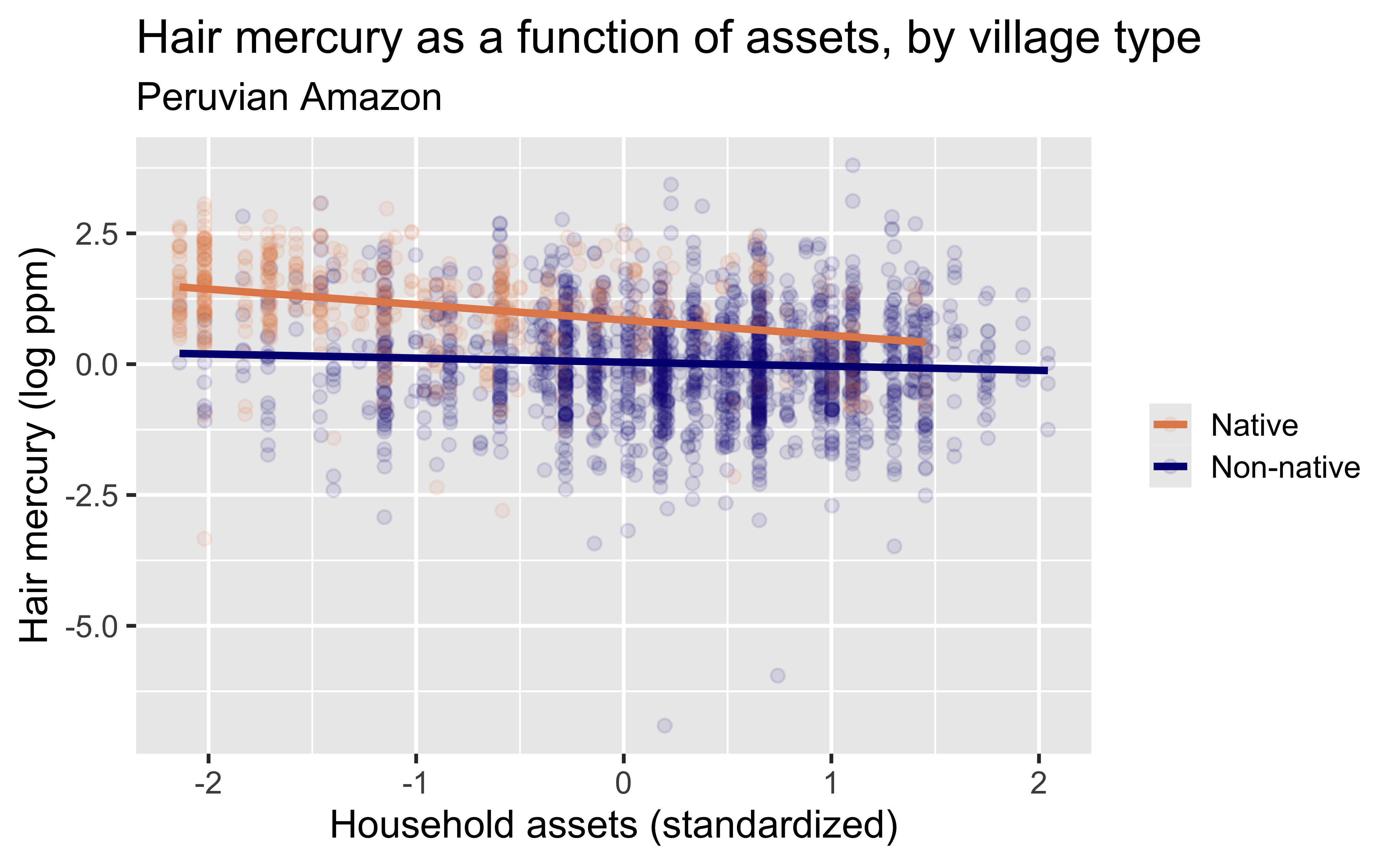
This figure corresponds to the model
\[\text{lnHg}_i=\beta_0+\beta_1 \text{sdas}_i + \beta_2 \text{nn}_i + \beta_3 \text{nn}_i\text{sdas}_i + \varepsilon_i,\]
where \(\text{lnHg}_i\) represents log hair mercury for subject \(i\), \(\text{sdas}_i\) represents standardized assets, \(\text{nn}_i=1\) if an individual lives in a non-native community and \(\text{nn}_i=0\) otherwise, and \(\text{nn}_i\text{sdas}_i\) is the interaction between assets and community status. (The interaction allows the slope of the line to differ across community status.)
A natural question is whether the slopes of these lines are significantly different – do we have evidence of different relationships between assets and hair mercury for those living in native and non-native communities?
From model to two lines
Full interaction model
\[\text{lnHg}_i=\beta_0+\beta_1 \text{sdas}_i + \beta_2 \text{nn}_i + \beta_3 \text{nn}_i\text{sdas}_i + \varepsilon_i\]
Fitted model
\[\widehat{\text{lnHg}}_i=\widehat{\beta}_0+\widehat{\beta}_1 \text{sdas}_i + \widehat{\beta}_2 \text{nn}_i + \widehat{\beta}_3 \text{nn}_i\text{sdas}_i\]
This gives two separate lines, one for each group:
Native
\[\widehat{\text{lnHg}}_i=\widehat{\beta}_0+\widehat{\beta}_1 \text{sdas}_i\]
Non-Native
\[\widehat{\text{lnHg}}_i=(\widehat{\beta}_0+\widehat{\beta}_2) + (\widehat{\beta}_1 + \widehat{\beta}_3) \text{sdas}_i\]
linear_reg() %>%
  set_engine("lm") %>%
  fit(lhairHg ~ assets_sc + native_cat + assets_sc*native_cat,
      data = mercury) %>%
  tidy()
# A tibble: 4 × 5
term estimate std.error statistic p.value
<chr> <dbl> <dbl> <dbl> <dbl>
1 (Intercept) 0.845 0.0575 14.7 9.93e-47
2 assets_sc -0.295 0.0430 -6.85 9.33e-12
3 native_catNon-native -0.807 0.0626 -12.9 9.10e-37
4 assets_sc:native_catNon-… 0.217 0.0519 4.18 2.99e- 5Native: \(\widehat{\text{lnHg}}_i=0.845 -0.295x_i\)
Non-Native: \(\widehat{\text{lnHg}}_i=(0.845-0.807) + (-0.295+0.217) x_i=0.038-0.078x_i\)
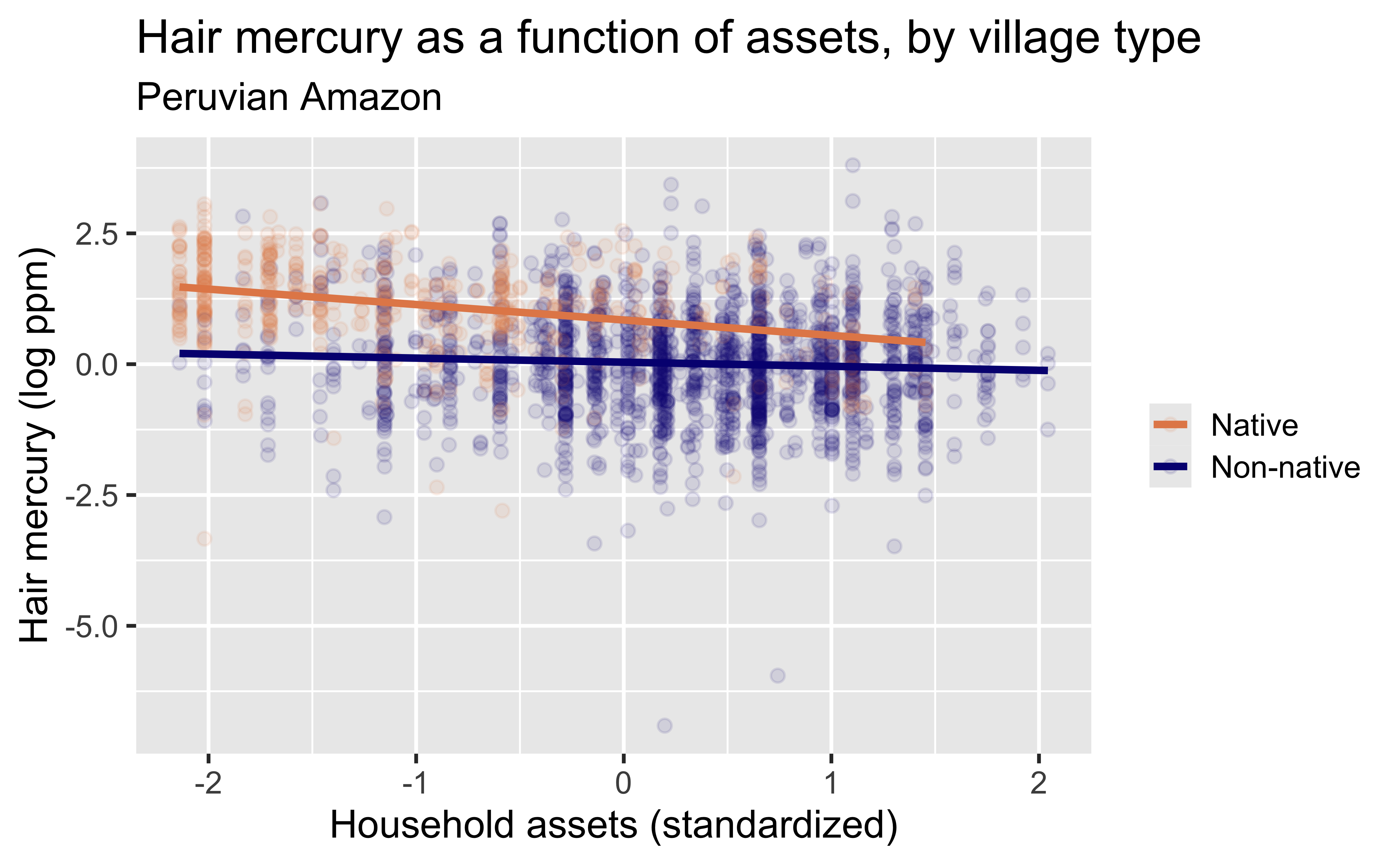
You can see that at the mean asset level (\(\text{sdas}_i=0\)), those in non-native communities have lower hair Hg levels, and in native communities we see a stronger relationship between assets and hair Hg, with little change in hair Hg as a function of assets in non-native communities, but a decrease with increasing assets in native communities.
Comparing model fit
Let’s fit the assets-only model and compare it to the fit of this model.
fit1 <-
  linear_reg() %>%
  set_engine("lm") %>%
  fit(lhairHg ~ assets_sc,
      data = mercury)

fit2 <-
  linear_reg() %>%
  set_engine("lm") %>%
  fit(lhairHg ~ assets_sc + native_cat + assets_sc*native_cat,
      data = mercury)

fit1 %>% glance() %>% print(width = Inf)
# A tibble: 1 × 12
r.squared adj.r.squared sigma statistic p.value df logLik
<dbl> <dbl> <dbl> <dbl> <dbl> <dbl> <dbl>
1 0.106 0.106 1.02 274. 3.90e-58 1 -3316.
AIC BIC deviance df.residual nobs
<dbl> <dbl> <dbl> <int> <int>
1 6638. 6655. 2407. 2298 2300# A tibble: 1 × 12
r.squared adj.r.squared sigma statistic p.value df logLik
<dbl> <dbl> <dbl> <dbl> <dbl> <dbl> <dbl>
1 0.208 0.207 0.964 201. 1.28e-115 3 -3177.
AIC BIC deviance df.residual nobs
<dbl> <dbl> <dbl> <int> <int>
1 6365. 6394. 2134. 2296 2300Adjusted \(R^2\)
0.106 ➔ 0.207
assets-only → with community status + interaction
Adjusted \(R^2\) is preferred to standard \(R^2\) in a model with more than one predictor:
- \(R^2\) can never decrease when more variables are added, so it can be suboptimal at identifying predictors that are not helpful.
- Adjusted \(R^2\) adds a penalty for having “too many” variables in a model and is preferred in multi-predictor settings.
Evaluating the interaction term
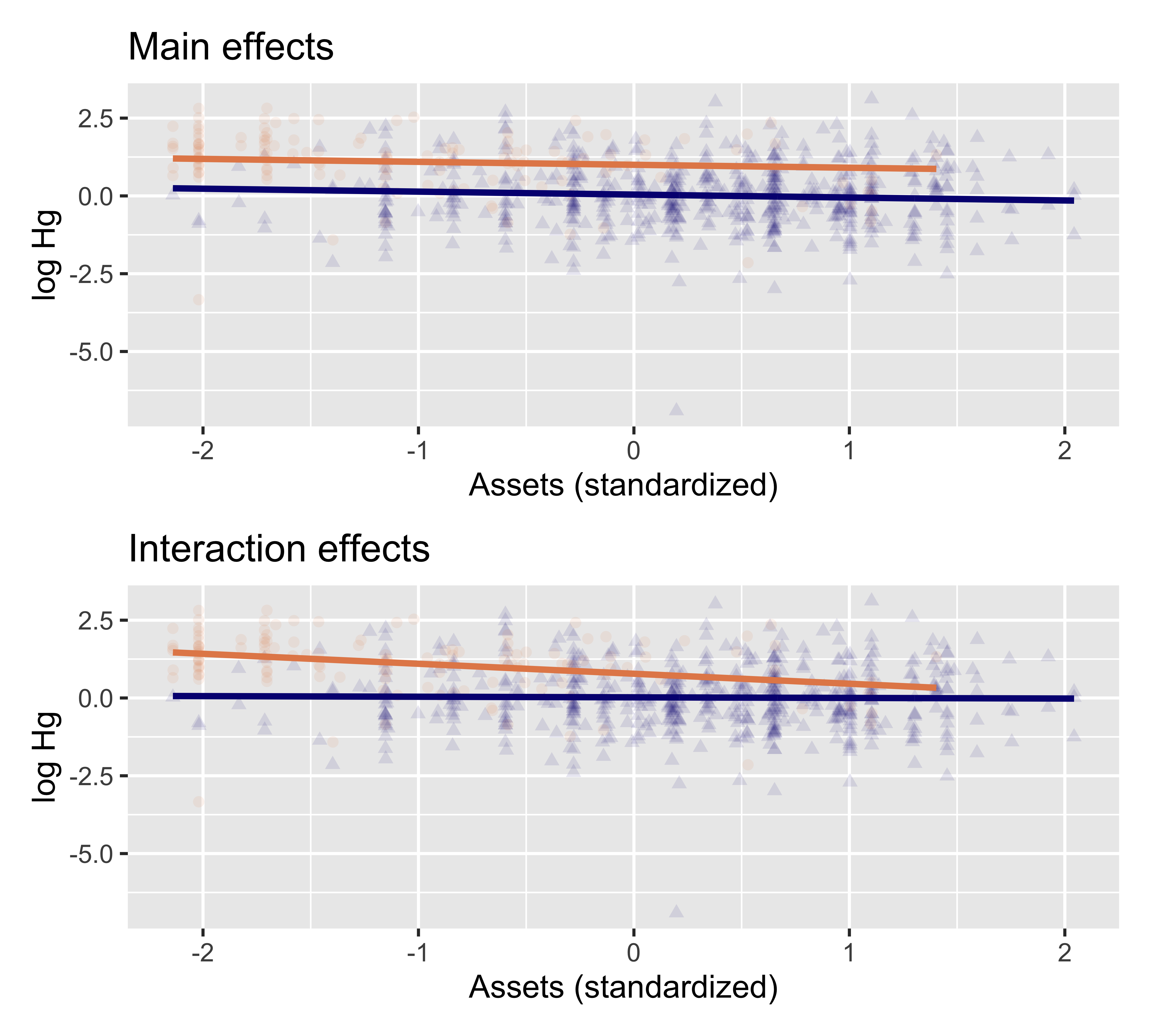
These plots illustrate the difference in the “main effects” model without any interaction term (top), and the interaction model (bottom). We want to evaluate how strongly the data support the need for different slopes to describe the assets-hair Hg relationship across community types. How might we do this?
Terminology: main effects and interactions
Recall our model: \[\text{lnHg}_i=\beta_0+\beta_1 \text{sdas}_i + \beta_2 \text{nn}_i + \beta_3 \text{nn}_i\text{sdas}_i + \varepsilon_i\]
Main effect
The effect of a predictor on its own, ignoring how it might depend on another variable.
- \(\beta_1\): the effect of assets when \(\text{nn}_i=0\), i.e. for the reference/native group
- \(\beta_2\): the effect of community type when \(\text{sdas}_i=0\), i.e. at mean assets
Interaction effect
The effect of one predictor depends on the value of another predictor.
- \(\beta_3\): how much the slope on assets changes when moving from native to non-native communities
An interaction answers: “does the relationship between assets and hair Hg differ by community type?”
If we need \(\beta_3\) in the model, assets and community status interact – the assets–mercury relationship is not the same in native vs. non-native communities, and we cannot describe the effect of assets with a single slope for everyone.
Evaluating the interaction term
We can conduct a formal hypothesis test of whether the interaction term improves our model \(\text{lnHg}_i=\beta_0+\beta_1 \text{sdas}_i + \beta_2 \text{nn}_i + \beta_3 \text{nn}_i\text{sdas}_i + \varepsilon_i\) by evaluating \(H_0: \beta_3=0\) against the alternative \(H_0: \beta_3 \neq 0\).
# A tibble: 4 × 7
  term   estimate std.error statistic  p.value conf.low conf.high
  <chr>     <dbl>     <dbl>     <dbl>    <dbl>    <dbl>     <dbl>
1 (Inte…    0.845    0.0575     14.7  9.93e-47    0.732     0.958
2 asset…   -0.295    0.0430     -6.85 9.33e-12   -0.379    -0.210
3 nativ…   -0.807    0.0626    -12.9  9.10e-37   -0.929    -0.684
4 asset…    0.217    0.0519      4.18 2.99e- 5    0.115     0.319
If we look at the last line of output, corresponding to the interaction term, we see that the p-value is quite small, which leads us to reject the null hypothesis and conclude that the interaction term does add to the model fit. So we do need to have separate slopes for assets by community type.
Adding sex to the model
Another variable that may help explain variability in hair Hg levels is sex. Let’s add it to see if that helps (note \(male_i=1\) if male and 0 if not). Our model now is \[\text{lnHg}_i=\beta_0+\beta_1 \text{sdas}_i + \beta_2 \text{nn}_i + \beta_3 \text{nn}_i\text{sdas}_i + \beta_4\text{male}_i+ \varepsilon_i\]
fit3 <-
  linear_reg() %>%
  set_engine("lm") %>%
  fit(lhairHg ~ assets_sc + native_cat + assets_sc*native_cat + sex_cat,
      data = mercury)
fit3 %>% tidy(conf.int=TRUE)
# A tibble: 5 × 7
term estimate std.error statistic p.value conf.low conf.high
<chr> <dbl> <dbl> <dbl> <dbl> <dbl> <dbl>
1 (Inte… 0.847 0.0602 14.1 3.61e-43 0.729 0.965
2 asset… -0.295 0.0430 -6.85 9.66e-12 -0.379 -0.210
3 nativ… -0.807 0.0627 -12.9 1.08e-36 -0.930 -0.684
4 sex_c… -0.00460 0.0420 -0.109 9.13e- 1 -0.0870 0.0778
5 asset… 0.217 0.0519 4.18 3.04e- 5 0.115 0.319 So the adjusted \(R^2\) changed little from 0.207 in the model without male sex. In addition, we see that the standard error of the sex coefficient in the model is large relative to its estimate, and the p-value is 0.9. So the sex term isn’t adding to our model fit or predictive ability.
Adding age to the model
Age in years, \(age_i\) is another potentially important predictor.
Dropping the sex term and adding age, our model now is \[\text{lnHg}_i=\beta_0+\beta_1 \text{sdas}_i + \beta_2 \text{nn}_i + \beta_3 \text{nn}_i\text{sdas}_i + \beta_5\text{age}_i+ \varepsilon_i\]
fit4 <-
  linear_reg() %>%
  set_engine("lm") %>%
  fit(lhairHg ~ assets_sc + native_cat + assets_sc*native_cat + age,
      data = mercury)
fit4 %>% tidy(conf.int=TRUE)
# A tibble: 5 × 7
term estimate std.error statistic p.value conf.low conf.high
<chr> <dbl> <dbl> <dbl> <dbl> <dbl> <dbl>
1 (Inte… 0.612 0.0647 9.46 7.32e-21 0.485 0.739
2 asset… -0.292 0.0425 -6.86 9.03e-12 -0.375 -0.208
3 nativ… -0.799 0.0618 -12.9 6.40e-37 -0.920 -0.677
4 age 0.00922 0.00123 7.50 8.87e-14 0.00681 0.0116
5 asset… 0.201 0.0513 3.91 9.40e- 5 0.100 0.301 Now the adjusted \(R^2\) has increased from 0.207, and we see that the p-value for age is quite small. We reject \(H_0: \beta_5=0\) and conclude that age is improving our model. Next we address how to interpret the coefficient in this setting.
Interpreting terms in multiple regression
Our model is \[\text{lnHg}_i=\beta_0+\beta_1 \text{sdas}_i + \beta_2 \text{nn}_i + \beta_3 \text{nn}_i\text{sdas}_i + \beta_5\text{age}_i+ \varepsilon_i\]
# A tibble: 5 × 7
  term   estimate std.error statistic  p.value conf.low conf.high
  <chr>     <dbl>     <dbl>     <dbl>    <dbl>    <dbl>     <dbl>
1 (Inte…  0.612     0.0647       9.46 7.32e-21  0.485      0.739
2 asset… -0.292     0.0425      -6.86 9.03e-12 -0.375     -0.208
3 nativ… -0.799     0.0618     -12.9  6.40e-37 -0.920     -0.677
4 age     0.00922   0.00123      7.50 8.87e-14  0.00681    0.0116
5 asset… 0.201 0.0513 3.91 9.40e- 5 0.100 0.301 Our fitted model is
\[\widehat{\text{lnHg}}_i=0.612 - 0.292 \text{sdas}_i - 0.799 \text{nn}_i + 0.201 \text{nn}_i \text{sdas}_i + 0.00922 \text{age}_i\]
The interpretation of the age term in our model is a little more complicated than the interpretation we had for assets in the assets-only model, but we still have two separate lines for community types.
Our fitted model is
\[\widehat{\text{lnHg}}_i=0.612 - 0.292 \text{sdas}_i - 0.799 \text{nn}_i + 0.201 \text{nn}_i \text{sdas}_i + 0.00922 \text{age}_i\] The slope coefficient for age in the log transformed model is 0.00922, meaning the log mercury difference between people whose ages are one year apart is predicted to be 0.00922 (95% CI=(0.00681,0.0116)) log ppm, if we hold all the other predictors in the model constant.
\[ \begin{aligned} \log(\text{hair Hg for age}_i+1, \text{sdas}_i, \text{nn}_i) &- \log(\text{hair Hg for age}_i, \text{sdas}_i, \text{nn}_i) = \\ & \Big[0.612 - 0.292\,\text{sdas}_i - 0.799\,\text{nn}_i + 0.201\,\text{nn}_i\text{sdas}_i + 0.00922(\text{age}_i+1)\Big] \\ & - \Big[0.612 - 0.292\,\text{sdas}_i - 0.799\,\text{nn}_i + 0.201\,\text{nn}_i\text{sdas}_i + 0.00922\,\text{age}_i\Big] \\ &= 0.00922 \end{aligned} \]
So then \[ \begin{aligned} \log(\text{hair Hg for age}_i+1, \text{sdas}_i, \text{nn}_i) - \log(\text{hair Hg for age}_i, \text{sdas}_i, \text{nn}_i) & = 0.00922 \\ \log\left(\frac{\text{hair Hg for age}_i+1, \text{sdas}_i, \text{nn}_i}{\text{hair Hg for age}_i, \text{sdas}_i, \text{nn}_i}\right) &= 0.00922 \\ e^{\log\left(\frac{\text{hair Hg for age}_i+1, \text{sdas}_i, \text{nn}_i}{\text{hair Hg for age}_i, \text{sdas}_i, \text{nn}_i}\right)} &= e^{0.00922} \\ \frac{\text{hair Hg for age}_i+1, \text{sdas}_i, \text{nn}_i}{\text{hair Hg for age}_i, \text{sdas}_i, \text{nn}_i} = 1.01 \end{aligned} \]
For residents who are one year older, at a fixed asset level and community status, the hair Hg is expected to be higher, on average, by a factor of 1.01.
1.01?
How can an an increase by a factor of 1.01 be significant? The issue here is scale – age is in years, but we don’t necessarily expect massive changes in mercury levels over a one-year period. Let’s consider a ten-year difference in age instead by creating an age variable that measures age in decades instead of years.
mercury <- mercury %>%
  mutate(age10 = age / 10)
fit5 <-
  linear_reg() %>%
  set_engine("lm") %>%
  fit(lhairHg ~ assets_sc + native_cat + assets_sc*native_cat + age10,
      data = mercury)
fit5 %>% tidy(conf.int=TRUE,exponentiate=TRUE)
# A tibble: 5 × 7
term estimate std.error statistic p.value conf.low conf.high
<chr> <dbl> <dbl> <dbl> <dbl> <dbl> <dbl>
1 (Inte… 1.84 0.0647 9.46 7.32e-21 1.62 2.09
2 asset… 0.747 0.0425 -6.86 9.03e-12 0.687 0.812
3 nativ… 0.450 0.0618 -12.9 6.40e-37 0.399 0.508
4 age10 1.10 0.0123 7.50 8.87e-14 1.07 1.12
5 asset… 1.22 0.0513 3.91 9.40e- 5 1.11 1.35 For residents who are ten years older, at a fixed asset level and community status, hair Hg is expected to be higher, on average, by a factor of
1.10
(95% CI: 1.07, 1.12)
Interpretation of All Estimates
We scaled age by 10, so our model is now \[\text{lnHg}_i=\beta_0+\beta_1 \text{sdas}_i + \beta_2 \text{nn}_i + \beta_3 \text{nn}_i\text{sdas}_i + \beta_5\frac{\text{age}_i}{10}+ \varepsilon_i\]
# A tibble: 5 × 7
  term   estimate std.error statistic  p.value conf.low conf.high
  <chr>     <dbl>     <dbl>     <dbl>    <dbl>    <dbl>     <dbl>
1 (Inte…    1.84     0.0647      9.46 7.32e-21    1.62      2.09
2 asset…    0.747    0.0425     -6.86 9.03e-12    0.687     0.812
3 nativ…    0.450    0.0618    -12.9  6.40e-37    0.399     0.508
4 age10     1.10     0.0123      7.50 8.87e-14    1.07      1.12
5 asset… 1.22 0.0513 3.91 9.40e- 5 1.11 1.35 Assets slope — Native
Holding age constant, each additional SD of assets in a native community is associated with hair Hg lower, on average, by a factor of 0.75.
Assets slope — Non-native
Holding age constant, each additional SD of assets in a non-native community is associated with hair Hg lower, on average, by a factor of \(e^{-0.292+0.201}=e^{-0.091}=\) 0.91.
Note: that’s from the figures on the log scale; if you do the math from this (exponentiated) table it’s just \((0.747)(1.22)=0.91\)
Interpretation of All Estimates
Our model is \[\text{lnHg}_i=\beta_0+\beta_1 \text{sdas}_i + \beta_2 \text{nn}_i + \beta_3 \text{nn}_i\text{sdas}_i + \beta_5\frac{\text{age}_i}{10}+ \varepsilon_i\]
# A tibble: 5 × 7
  term   estimate std.error statistic  p.value conf.low conf.high
  <chr>     <dbl>     <dbl>     <dbl>    <dbl>    <dbl>     <dbl>
1 (Inte…    1.84     0.0647      9.46 7.32e-21    1.62      2.09
2 asset…    0.747    0.0425     -6.86 9.03e-12    0.687     0.812
3 nativ…    0.450    0.0618    -12.9  6.40e-37    0.399     0.508
4 age10     1.10     0.0123      7.50 8.87e-14    1.07      1.12
5 asset… 1.22 0.0513 3.91 9.40e- 5 1.11 1.35 Age slope
At a fixed asset level and community status, residents ten years older are expected to have higher hair Hg, on average, by a factor of 1.10.
Main effect of native status
At the mean asset level, holding age constant, hair mercury in non-native communities is lower, on average, by a factor of 0.45 than in native communities.