Categorical Data and Contingency Tables

Introduction to Global Health Data Science

Prof. Amy Herring

Duke University
STA/GLHLTH 198 Fall 2026

Introduction to contingency tables

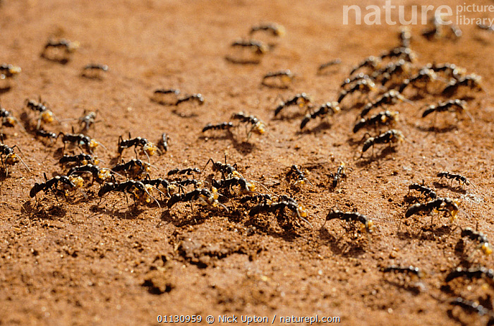
Recall our termite-raiding ant data

Recall our termite-raiding ant data:

	Carried Back	Carried Away	Not Carried
Lightly Injured	45	0	5
Heavily Injured	5	5	20

Contingency tables

A contingency table displays the relationship between two categorical variables.

Here, each observation is an ant. The variables are injury severity and carrying outcome.

Injury	Carried back	Carried away	Not carried	Total
Lightly injured	45	0	5	50
Heavily injured	5	5	20	30
Total	50	5	25	80

Dataset: one row per ant (subset of 15 rows)

Injury	Outcome
Lightly injured	Carried back
Lightly injured	Carried back
Lightly injured	Carried back
Lightly injured	Carried back
Lightly injured	Carried back
Lightly injured	Carried back
Lightly injured	Carried back
Heavily injured	Not carried
Lightly injured	Carried back
Heavily injured	Carried away
Heavily injured	Not carried
Heavily injured	Not carried
Heavily injured	Not carried
Lightly injured	Carried back
Lightly injured	Carried back

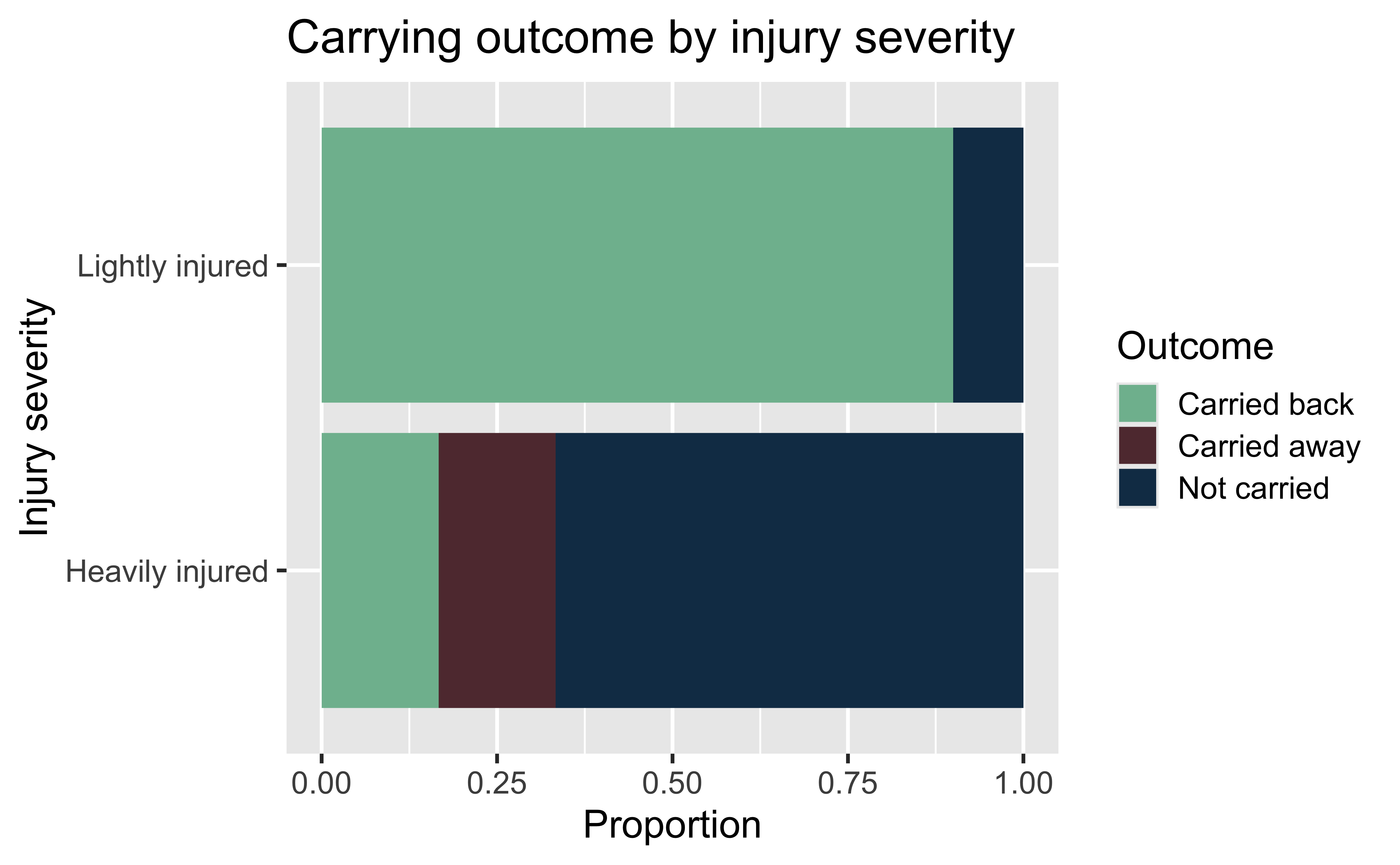
Visualizing injury severity and carrying outcome

• Plot
• Code

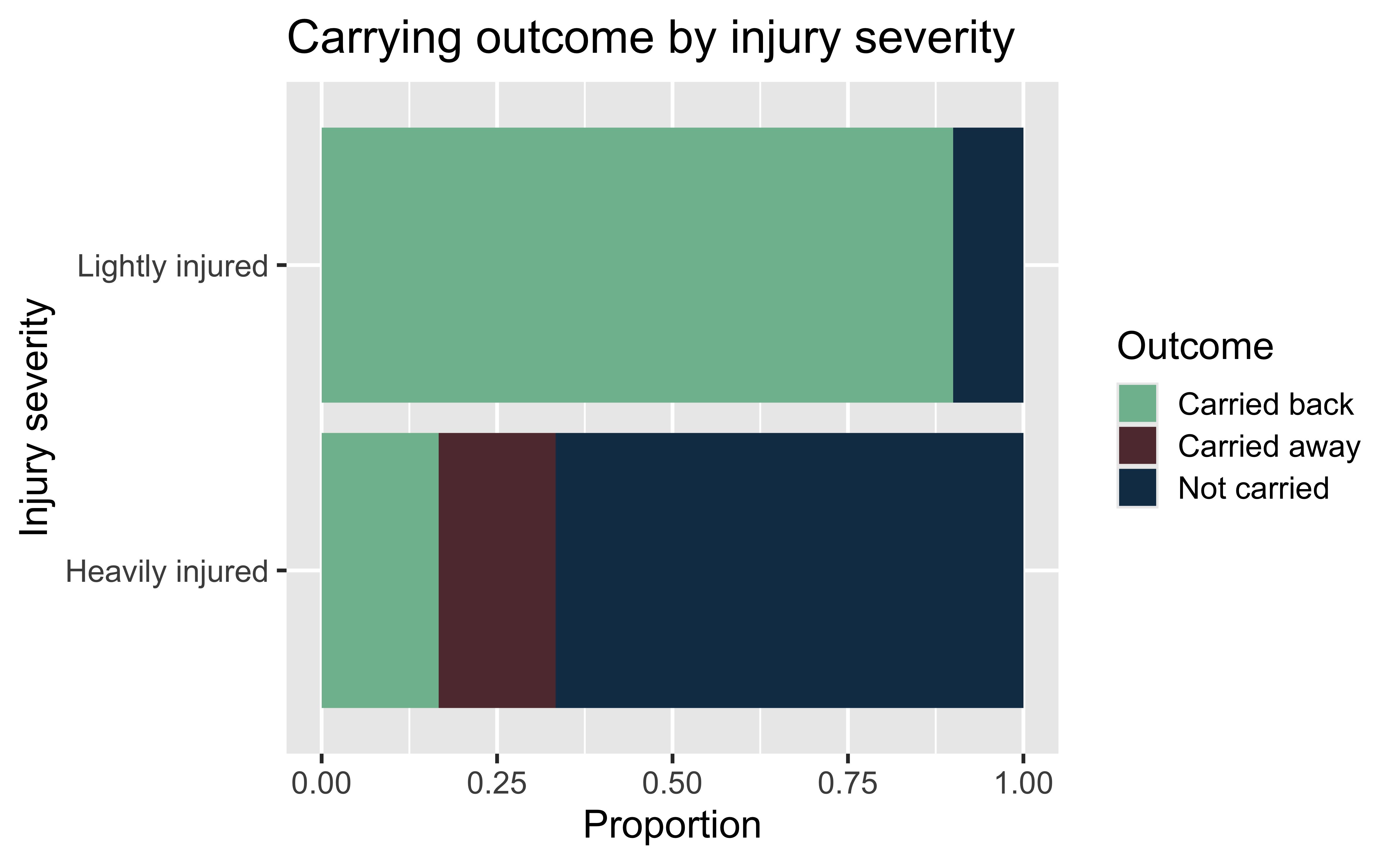
ants %>%
  ggplot(aes(y = Injury, fill = Outcome)) +
  geom_bar(position = position_fill(reverse = TRUE)) +
  #reverse equals true puts carried back on the left
  scale_y_discrete(limits = c("Heavily injured", "Lightly injured")) + #this line puts light injury as the top row to match our contingency table formatting
  labs(x = "Proportion", y = "Injury severity",
       title = "Carrying outcome by injury severity") +
  scale_fill_manual(values = c(
    "Carried back" = "#7FBB9E",  # Neptune Green
    "Carried away" = "#60373D",  # Red Mahogany
    "Not carried" = "#133955"   # Poseidon
  ))

Are injury severity and carrying outcome related?

If there were no association, we would expect approximately the same proportions of the three outcomes in both injury groups.

Are the differences in this sample evidence of an association, or could they reflect random variation?

Typical questions with \(r\times c\) contingency tables

• Is there an association between the row variable and the column variable?
  • Here, \(r=2\) injury groups and \(c=3\) carrying outcomes.
• How strong is the association?

\(H_0:\) injury severity and carrying outcome are independent.

\(H_A:\) injury severity and carrying outcome are associated.

Tests for association

Fisher’s exact test

Fisher’s exact test

Fisher’s exact test assesses whether two categorical variables are associated.

It does not require large expected cell counts, so it is useful when a contingency table includes small counts, as is the case here.

The test can be computationally expensive for large tables.

How Fisher’s exact test works

We condition on the observed margins, the row and column totals:

• 50 lightly injured ants and 30 heavily injured ants;
• 50 carried back, 5 carried away, and 25 not carried.

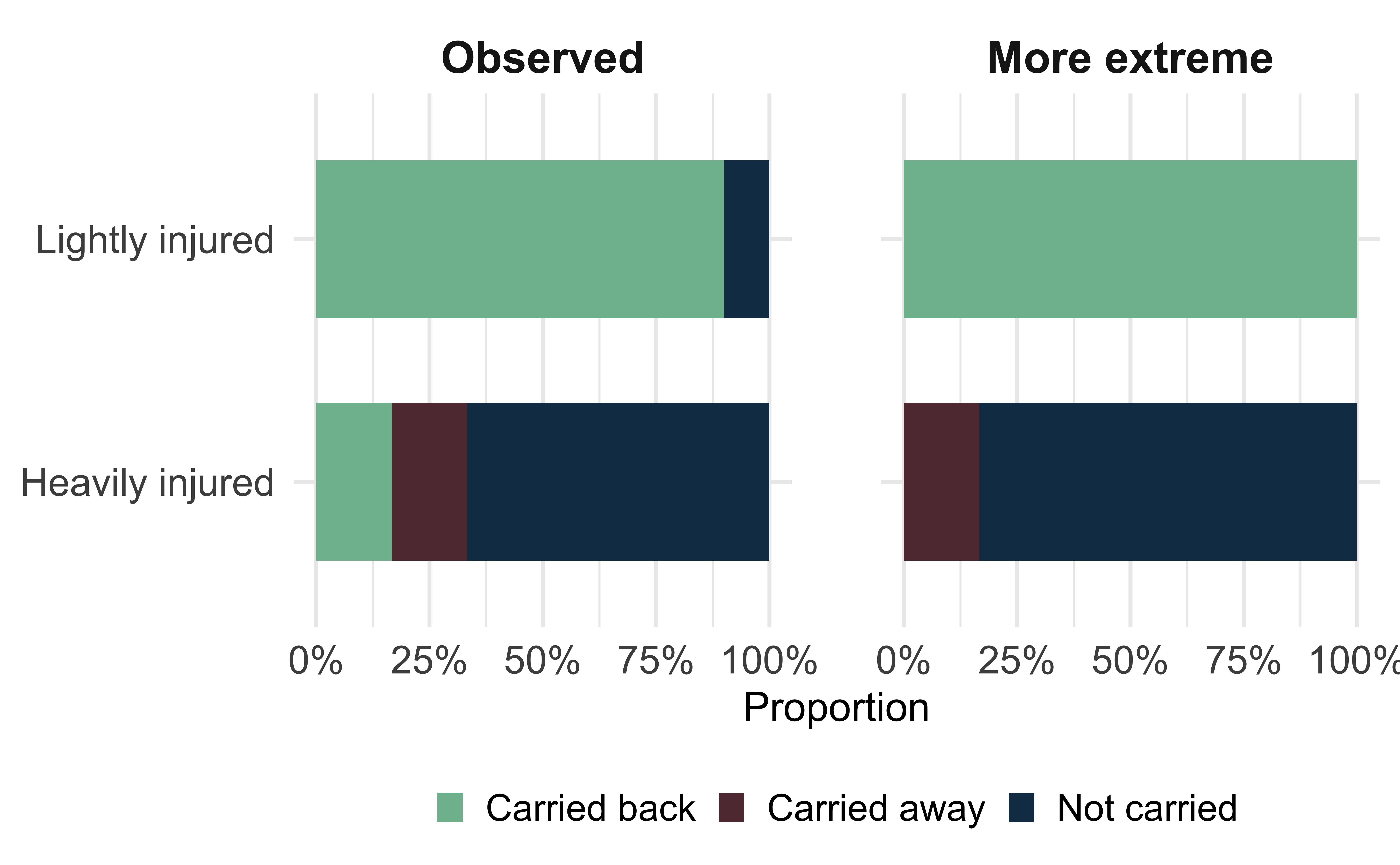
Consider all possible tables with those same margins. Under \(H_0\), each table has a probability.

The two-sided p-value sums the probabilities of tables whose null probabilities are less than or equal to that of our observed table.

R documentation for the fixed-margins test and probability ordering: https://stat.ethz.ch/R-manual/R-devel/library/stats/html/fisher.test.html

Tables with the same margins

Observed table

Injury	Carried back	Carried away	Not carried	Total
Lightly injured	45	0	5	50
Heavily injured	5	5	20	30
Total	50	5	25	80

A more extreme table with the same margins

Injury	Carried back	Carried away	Not carried	Total
Lightly injured	50	0	0	50
Heavily injured	0	5	25	30
Total	50	5	25	80

Fisher’s exact test for the ant data

ant_tab #view the table

#>                  
#>                   Carried back Carried away Not carried
#>   Lightly injured           45            0           5
#>   Heavily injured            5            5          20

ant_fisher <- fisher.test(ant_tab)
ant_fisher

#> 
#>  Fisher's Exact Test for Count Data
#> 
#> data:  ant_tab
#> p-value = 2.576e-11
#> alternative hypothesis: two.sided

The p-value is approximately \(2.58\times10^{-11}\).

There is strong evidence of an association between injury severity and carrying outcome.

\(\chi^2\) (chi-squared) test

\(\chi^2\) test

The chi-squared test compares observed cell counts with the counts expected if \(H_0\) were true.

Its p-value uses an approximation that depends on the expected counts. For this course, use the guideline that every expected cell count should be at least 5.

We will calculate the expected counts and test statistic for the ant table, then check that guideline.

Marginal probabilities

Injury	Carried back	Carried away	Not carried	Total
Lightly injured	45	0	5	50
Heavily injured	5	5	20	30
Total	50	5	25	80

Injury severity:

• \(P(\text{lightly injured})=50/80\)

• \(P(\text{heavily injured})=30/80\)

Carrying outcome:

• \(P(\text{back})=50/80\)

• \(P(\text{away})=5/80\)

• \(P(\text{not carried})=25/80\).

Expected counts under independence

Suppose \(H_0\) is true: injury severity and carrying outcome are independent.

What is the probability that an ant is lightly injured and carried back? Recall that under independence, \(P(A \cap B)=P(A)P(B)\).

\[ P(\text{lightly injured and carried back}) =P(\text{lightly injured})P(\text{carried back}) =\frac{50}{80}\times\frac{50}{80}. \]

From probabilities to expected counts

Multiply the probability by the number of ants:

\[ E_{\text{light, back}} =\frac{50}{80}\times\frac{50}{80}\times80 =31.25. \]

In general, for any cell:

\[ E=\frac{\text{row total}\times\text{column total}}{\text{grand total}}. \]

Building the expected table

\(E_{\text{light, back}}=\frac{50\times50}{80}=31.25\)

Injury	Carried back	Carried away	Not carried	Total
Lightly injured	31.25			50
Heavily injured				30
Total	50	5	25	80

Building the expected table

\(E_{\text{light, away}}=\frac{50\times5}{80}=3.125\)

Injury	Carried back	Carried away	Not carried	Total
Lightly injured	31.25	3.125		50
Heavily injured				30
Total	50	5	25	80

Building the expected table

\(E_{\text{light, not carried}}=50-31.25-3.125=15.625\)

Injury	Carried back	Carried away	Not carried	Total
Lightly injured	31.250	3.125	15.625	50
Heavily injured				30
Total	50	5	25	80

Building the expected table

\(E_{\text{heavy, back}}=50-31.25=18.75\)

Injury	Carried back	Carried away	Not carried	Total
Lightly injured	31.250	3.125	15.625	50
Heavily injured	18.75			30
Total	50	5	25	80

Building the expected table

\(E_{\text{heavy, away}}=5-3.125=1.875\)

Injury	Carried back	Carried away	Not carried	Total
Lightly injured	31.250	3.125	15.625	50
Heavily injured	18.750	1.875		30
Total	50	5	25	80

Building the expected table

\(E_{\text{heavy, not carried}}=30-18.75-1.875=9.375\)

Injury	Carried back	Carried away	Not carried	Total
Lightly injured	31.250	3.125	15.625	50
Heavily injured	18.750	1.875	9.375	30
Total	50	5	25	80

The expected table under \(H_0\)

If injury severity and carrying outcome were independent, these would be the expected counts:

Injury	Carried back	Carried away	Not carried	Total
Lightly injured	31.250	3.125	15.625	50
Heavily injured	18.750	1.875	9.375	30
Total	50	5	25	80

Comparing observed and expected tables

Observed

Injury	Carried back	Carried away	Not carried	Total
Lightly injured	45	0	5	50
Heavily injured	5	5	20	30
Total	50	5	25	80

Expected under \(H_0\)

Injury	Carried back	Carried away	Not carried	Total
Lightly injured	31.250	3.125	15.625	50
Heavily injured	18.750	1.875	9.375	30
Total	50	5	25	80

The observed table differs from the expected table. How can we summarize those differences?

Comparing observed and expected tables

Observed

Injury	Carried back	Carried away	Not carried	Total
Lightly injured	45	0	5	50
Heavily injured	5	5	20	30
Total	50	5	25	80

Expected under \(H_0\)

Injury	Carried back	Carried away	Not carried	Total
Lightly injured	31.250	3.125	15.625	50
Heavily injured	18.750	1.875	9.375	30
Total	50	5	25	80

The \(\chi^2\) test compares observed frequencies, \(O\), with expected frequencies, \(E\), in each cell.

Comparing observed and expected tables

Observed

Injury	Carried back	Carried away	Not carried	Total
Lightly injured	45	0	5	50
Heavily injured	5	5	20	30
Total	50	5	25	80

Expected under \(H_0\)

Injury	Carried back	Carried away	Not carried	Total
Lightly injured	31.250	3.125	15.625	50
Heavily injured	18.750	1.875	9.375	30
Total	50	5	25	80

Large differences, \(O-E\), provide evidence against \(H_0\).

Comparing observed and expected tables

Observed

Injury	Carried back	Carried away	Not carried	Total
Lightly injured	45	0	5	50
Heavily injured	5	5	20	30
Total	50	5	25	80

Expected under \(H_0\)

Injury	Carried back	Carried away	Not carried	Total
Lightly injured	31.250	3.125	15.625	50
Heavily injured	18.750	1.875	9.375	30
Total	50	5	25	80

We square the differences, \((O-E)^2\), so that positive and negative differences do not cancel each other out.

Comparing observed and expected tables

Observed

Injury	Carried back	Carried away	Not carried	Total
Lightly injured	45	0	5	50
Heavily injured	5	5	20	30
Total	50	5	25	80

Expected under \(H_0\)

Injury	Carried back	Carried away	Not carried	Total
Lightly injured	31.250	3.125	15.625	50
Heavily injured	18.750	1.875	9.375	30
Total	50	5	25	80

We divide each squared difference by \(E\) to account for the scale of the expected count: \(\frac{(O-E)^2}{E}\)

The \(\chi^2\) test statistic

Our test statistic is

\[ X^2=\sum_{i=1}^{rc}\frac{(O_i-E_i)^2}{E_i}. \]

Here, there are \(r\times c=2\times3=6\) cells, excluding the totals:

Observed

Injury	Carried back	Carried away	Not carried	Total
Lightly injured	45	0	5	50
Heavily injured	5	5	20	30
Total	50	5	25	80

Expected under \(H_0\)

Injury	Carried back	Carried away	Not carried	Total
Lightly injured	31.250	3.125	15.625	50
Heavily injured	18.750	1.875	9.375	30
Total	50	5	25	80

\[ X^2=\frac{(45-31.25)^2}{31.25} +\frac{(0-3.125)^2}{3.125} +\cdots+\frac{(20-9.375)^2}{9.375} =43.73. \]

Checking the expected counts

Injury	Carried back	Carried away	Not carried	Total
Lightly injured	31.250	3.125	15.625	50
Heavily injured	18.750	1.875	9.375	30
Total	50	5	25	80

The expected counts for carried away are 3.125 and 1.875, both below 5.

Use Fisher’s exact test for the main conclusion. The chi-squared calculations illustrate the method, but the large-sample approximation may be unreliable here.

The \(\chi^2\) distribution

• Under \(H_0\), the test statistic is approximately chi-squared when expected counts are sufficiently large.
• The degrees of freedom are \((r-1)(c-1)=(2-1)(3-1)=2\).
• The distribution is asymmetric and takes nonnegative values.
• Larger statistics provide more evidence against \(H_0\), so the p-value is an area in the right tail.

Calculating the \(\chi^2\) statistic in R

observed_chisq_statistic <- ants %>%
  specify(Injury ~ Outcome) %>%
  calculate(stat = "Chisq")

observed_chisq_statistic

#> Response: Injury (factor)
#> Explanatory: Outcome (factor)
#> # A tibble: 1 × 1
#>    stat
#>   <dbl>
#> 1  43.7

The statistic is approximately 43.7.

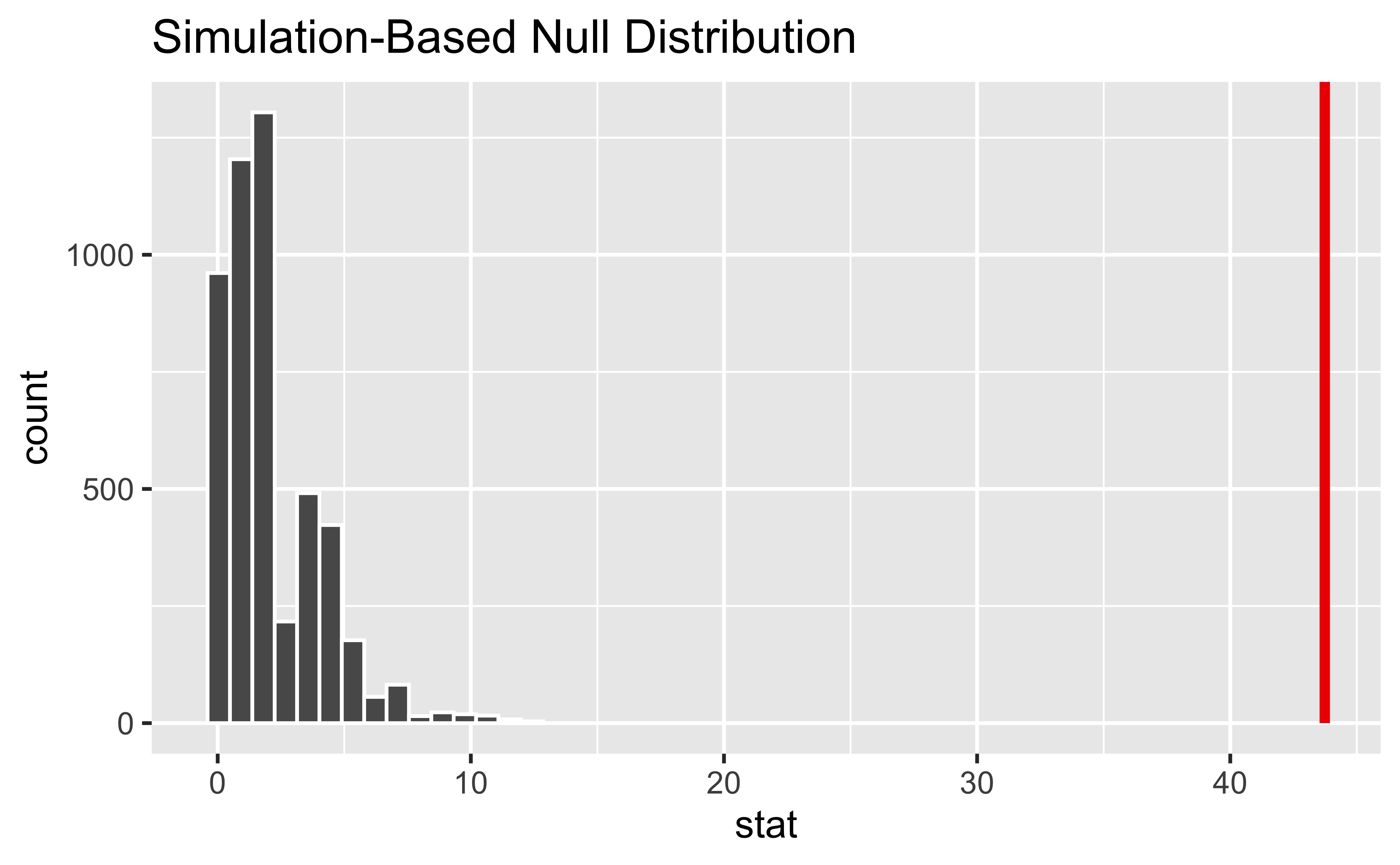
Simulating the null distribution

We can generate a null distribution by permuting carrying outcomes among the ants, keeping the margins fixed.

set.seed(1234)
null_distribution_simulated <- ants %>%
  specify(Injury ~ Outcome) %>%
  hypothesize(null = "independence") %>%
  generate(reps = 5000, type = "permute") %>%
  calculate(stat = "Chisq")

The theoretical null distribution

The theoretical approximation uses a \(\chi^2_2\) distribution.

ant_hypothesis <- ants %>%
  specify(Injury ~ Outcome) %>%
  hypothesize(null = "independence")

Remember that two expected counts are below 5. We will compare this approximation with the simulated null distribution.

Visualizing the simulated null distribution

• Plot
• Code

null_distribution_simulated %>%
  visualize() +
  shade_p_value(observed_chisq_statistic, direction = "greater")

Visualizing the theoretical null distribution

• Plot
• Code

ant_hypothesis %>%
  visualize(method = "theoretical") +
  shade_p_value(observed_chisq_statistic, direction = "greater")

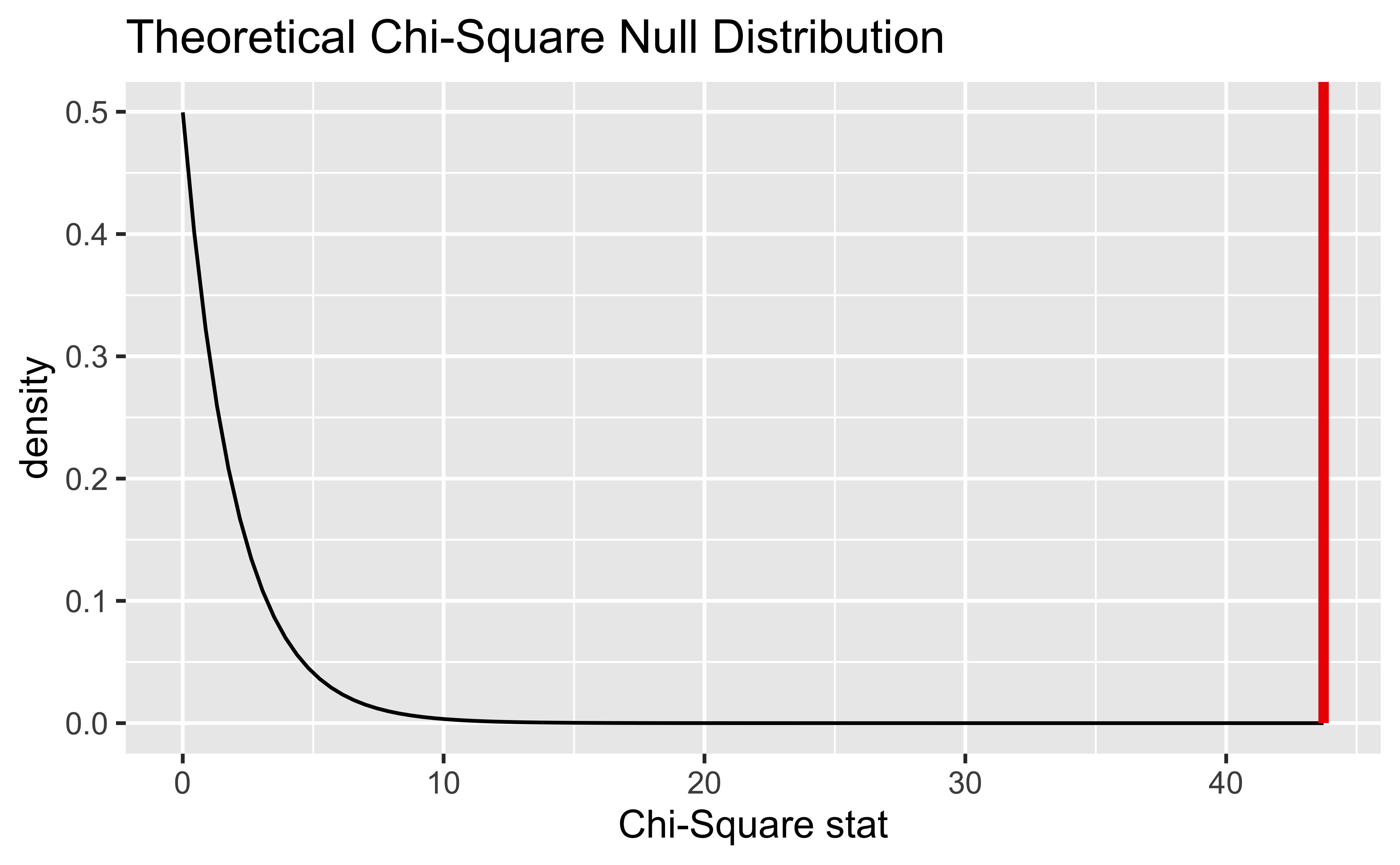
Comparing both null distributions

• Plot
• Code

null_distribution_simulated %>%
  visualize(method = "both") +
  shade_p_value(observed_chisq_statistic, direction = "greater")

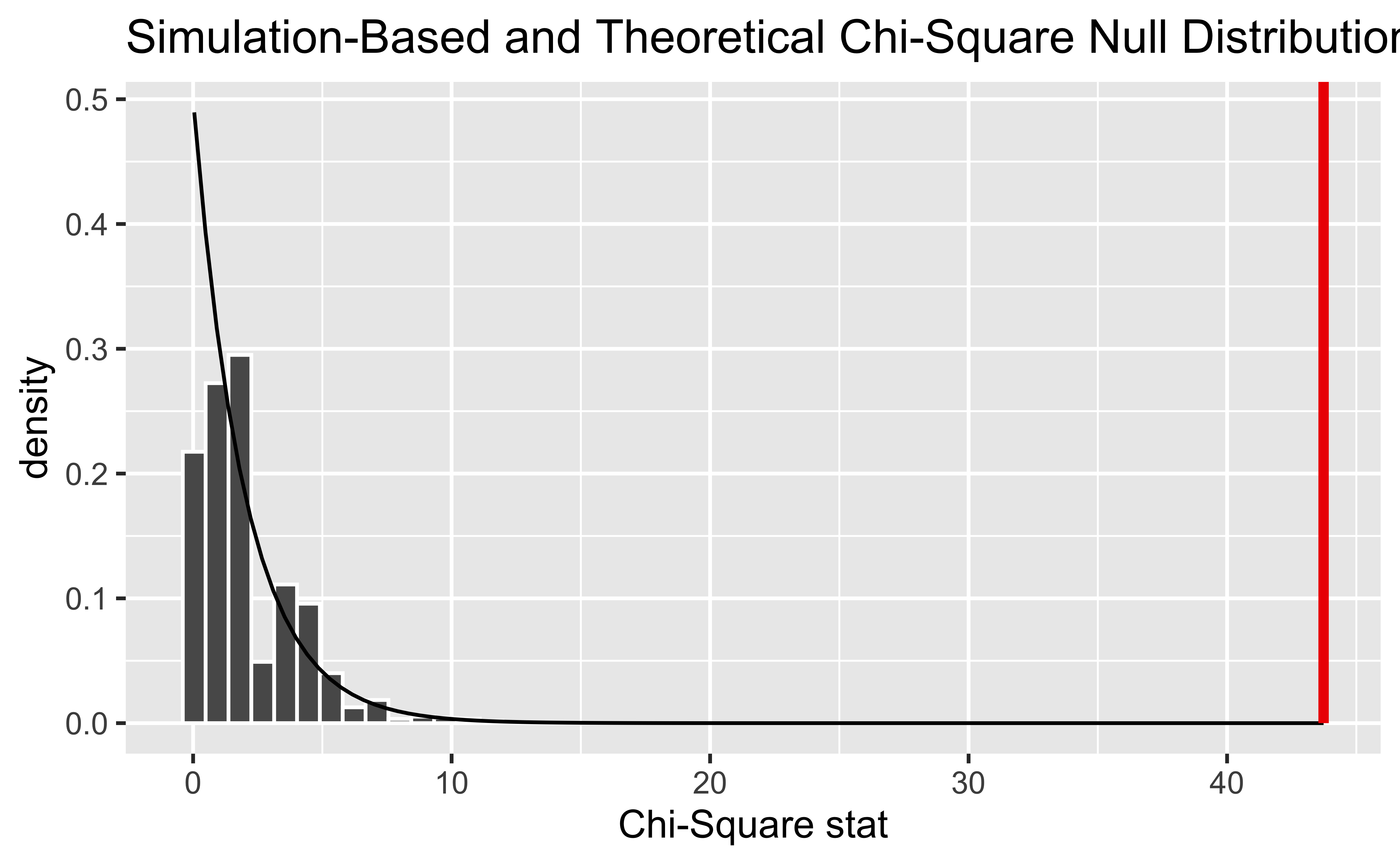
The chi-squared approximation for the ant data

# This returns an approximate p-value.
ant_chisq <- chisq.test(ant_tab, correct = FALSE)
ant_chisq

#> 
#>  Pearson's Chi-squared test
#> 
#> data:  ant_tab
#> X-squared = 43.733, df = 2, p-value = 3.187e-10

\(X^2=43.73\) on 2 degrees of freedom, with an approximate p-value of \(3.19\times10^{-10}\).

Because two expected counts are small, use the earlier Fisher p-value for inference. Both calculations suggest a strong association.

The warning about a potentially incorrect approximation is expected for these data. The global chunk settings suppress warnings on the slides, but the limitation is stated explicitly in the slide text. Yates’ correction applies only to 2 x 2 tables, not this 2 x 3 table. https://stat.ethz.ch/R-manual/R-devel/library/stats/html/chisq.test.html

A very small p-value and simulation

With 5,000 permutations, we may see no simulated statistics as large as 43.73. That does not mean the true p-value is zero.

n_extreme <- sum(
  null_distribution_simulated$stat >= observed_chisq_statistic$stat
)
p_sim <- (n_extreme + 1) / (nrow(null_distribution_simulated) + 1)
p_sim

#> [1] 0.00019996

If none are as extreme, this adjusted estimate is \(1/5001\approx0.0002\). Fisher’s exact test can resolve the much smaller p-value for this table.

How strong is the association?

The Odds Ratio

An odds ratio compares two groups that have a binary outcome.

For the ants, compare carried back with not carried back. The latter combines carried away and not carried.

Injury	Carried back	Not carried back	Total
Lightly injured	45	5	50
Heavily injured	5	25	30
Total	50	30	80

This asks whether injury severity is associated with being carried back. It uses all 80 ants, but it summarizes the original three outcomes as two.

Let \(B\) mean carried back and \(L\) mean lightly injured. Then \(\overline{L}\) means heavily injured.

What are the Odds?

The odds of an event compare how often it happens with how often it does not happen:

\[ \text{Odds of being carried back} =\frac{P(B)}{1-P(B)} =\frac{\text{number carried back}}{\text{number not carried back}}. \]

Injury	Carried back	Not carried back	Probability	Odds
Lightly injured	45	5	\(45/50=0.90\)	\(\frac{\frac{45}{50}}{\frac{5}{50}}=\frac{45}{5}=9\) to \(1\)
Heavily injured	5	25	\(5/30\approx0.17\)	\(\frac{\frac{5}{50}}{\frac{25}{50}}=\frac{5}{25}=1\) to \(5\)

For lightly injured ants, 9 to 1 odds means that for every one ant not carried back, nine were carried back.

The odds ratio (OR)

\[ OR=\frac{P(B\mid L)/[1-P(B\mid L)]} {P(B\mid \overline{L})/[1-P(B\mid \overline{L})]}. \]

The OR ranges from 0 to \(\infty\).

• \(OR=1\): the two groups have equal odds of being carried back.
• \(OR>1\): lightly injured ants have higher odds.
• \(OR<1\): lightly injured ants have lower odds.

Odds ratio from a contingency table

	Group 1	Group 2
Outcome present	\(a\)	\(b\)
Outcome absent	\(c\)	\(d\)

The estimated probabilities are

\[ \widehat P_1=\frac{a}{a+c}, \qquad \widehat P_2=\frac{b}{b+d}. \]

For Group 1, the probability of the outcome being absent is \(1-\widehat P_1=c/(a+c)\). Thus its odds are

\[ \frac{\widehat P_1}{1-\widehat P_1} = \frac{a/(a+c)}{c/(a+c)} = \frac{a}{c}. \]

Similarly, the odds for Group 2 are \(\dfrac{b/(b+d)}{d/(b+d)}=\dfrac{b}{d}\). Dividing the two odds gives

\[ \widehat{OR} = \frac{a/c}{b/d} = \frac{ad}{bc}. \]

Odds ratio for being carried back

The odds of being carried back are

\[ \text{Lightly injured: }\frac{45}{5}=9, \qquad \text{Heavily injured: }\frac{5}{25}=0.2. \]

\[ \widehat{OR}=\frac{9}{0.2}=45. \]

In this sample, lightly injured ants have 45 times the odds of being carried back compared with heavily injured ants.

This compares odds, rather than probabilities.

Odds ratio using the formula

Here, the outcome is carried back. “Not carried back” includes ants carried away or not carried at all.

	Lightly injured (Group 1)	Heavily injured (Group 2)
Carried back	\(a=45\)	\(b=5\)
Not carried back	\(c=5\)	\(d=25\)

Substitute these counts into the formula:

\[ \widehat{OR} =\frac{ad}{bc} =\frac{45(25)}{5(5)} =\frac{1125}{25} =45. \]

The odds of being carried back were 45 times as high for lightly injured ants as for heavily injured ants.

Creating the binary outcome in R

ants_binary <- ants %>%
  mutate(
    Carried_back = if_else(Outcome == "Carried back", "Yes", "No"),
    Carried_back = factor(Carried_back, levels = c("Yes", "No"))
  )

ant_binary_tab <- table(ants_binary$Injury, ants_binary$Carried_back)
ant_binary_tab

#>                  
#>                   Yes No
#>   Lightly injured  45  5
#>   Heavily injured   5 25

Rows are ordered lightly injured, heavily injured. Columns are ordered Yes, No. This makes the OR compare lightly injured with heavily injured ants.

Estimating an OR and a 95% confidence interval

ant_or_result <- fisher.test(ant_binary_tab)
ant_or_result

#> 
#>  Fisher's Exact Test for Count Data
#> 
#> data:  ant_binary_tab
#> p-value = 3.476e-11
#> alternative hypothesis: true odds ratio is not equal to 1
#> 95 percent confidence interval:
#>   10.29032 212.82087
#> sample estimates:
#> odds ratio 
#>   41.32031

The estimated OR (conditional MLE) is 41.3, with a 95% CI of (10.3, 212.8).

The CI excludes 1, providing evidence that the odds of being carried back differ by injury severity.

fisher.test() reports a conditional maximum likelihood estimate, which differs slightly from the sample cross-product estimate of 45.

Practice: pneumococcal serotypes and survival

Practice: the serotype data

A Scottish study examined the association between pneumococcal serotype and survival following infection.

Serotype	Survived	Died	Total
Serotype 10	37	7	44
Serotype 15	60	12	72
Serotype 20	97	9	106
Serotype 31	24	10	34
Total	218	38	256

1. Identify the two categorical variables and the dimensions of this table.
2. State the null and alternative hypotheses for a test of association.

Practice: expected counts

Serotype	Survived	Died	Total
Serotype 10	37	7	44
Serotype 15	60	12	72
Serotype 20	97	9	106
Serotype 31	24	10	34
Total	218	38	256

3. Calculate the expected number of deaths for serotype 31 under \(H_0\).
4. Calculate the other expected counts. Is the chi-squared approximation appropriate under our course guideline?
5. What are the degrees of freedom?

Expected survivors and deaths, respectively: Serotype 10: 37.46875, 6.53125. Serotype 15: 61.3125, 10.6875. Serotype 20: 90.265625, 15.734375. Serotype 31: 28.953125, 5.046875. All expected counts exceed 5. The degrees of freedom are 3.

Practice: enter the data in R

pneu_counts <- tibble(
  Serotype = rep(c("Serotype 10", "Serotype 15",
                  "Serotype 20", "Serotype 31"), each = 2),
  Survival = rep(c("Survived", "Died"), 4),
  n = c(37, 7, 60, 12, 97, 9, 24, 10)
)

pneu <- pneu_counts %>% uncount(n)
pneu_tab <- table(pneu$Serotype, pneu$Survival)

The dataset contains one row per person. pneu_tab contains the cell counts.

Practice: tests of association

6. Use Fisher’s exact test and the chi-squared test. Compare their conclusions and interpret the p-values in context.

# Run the tests, then interpret the results.
fisher.test(pneu_tab)
chisq.test(pneu_tab)

The chi-squared statistic is approximately 9.322 on 3 degrees of freedom, with p-value 0.02530. Fisher’s p-value is approximately 0.02658. Both provide evidence of an association at the 0.05 level.

Practice: odds ratio

7. Compare serotypes 20 and 31. Calculate the sample odds ratio for death, comparing serotype 20 with serotype 31.
8. Use R to obtain an odds ratio and 95% CI. Interpret them and explain whether the CI supports an association.

pneu_20_31 <- pneu %>%
  filter(Serotype %in% c("Serotype 20", "Serotype 31")) %>%
  mutate(
    Serotype = factor(Serotype, levels = c("Serotype 20", "Serotype 31")),
    Survival = factor(Survival, levels = c("Died", "Survived"))
  )

# Check the row and column order before interpreting the OR.
table(pneu_20_31$Serotype, pneu_20_31$Survival)
fisher.test(table(pneu_20_31$Serotype, pneu_20_31$Survival))

The sample OR is \((9\times24)/(97\times10)=0.2227\). R’s conditional OR is approximately 0.23, with 95% CI approximately (0.07, 0.69). Serotype 20 is associated with lower odds of death than serotype 31. The CI excludes 1. This comparison concerns odds, not risk.

Practice: another comparison

9. Compare serotypes 10 and 31 using Fisher’s exact test. What do you conclude?

pneu_10_31 <- pneu %>%
  filter(Serotype %in% c("Serotype 10", "Serotype 31"))

fisher.test(table(pneu_10_31$Serotype, pneu_10_31$Survival))

If you test several serotype pairs, consider how multiple comparisons affect the chance of a false positive.