Data Wrangling

Introduction to Global Health Data Science

Author

Affiliation

Amy Herring

Duke University
STA/GLHLTH 198 Fall 2026

Main Ideas

• Organizing our data according to a consistent set of “tidy” principles makes data easy to work with and leverages the ways R is effective.

• Often we need to wrangle our data in order to extract meaning (including creating new variables, calculating summary statistics, subsetting data, etc).

• Using only seven key verbs we can accomplish a wide variety of data wrangling tasks.

Tidy Principles

Tidy data have three related characteristics

1. Each variable forms a column.

2. Each observation forms a row.

3. Each value has its own cell.

Rural and Urban Patterns of Global Obesity

Obesity is a major risk factor for numerous non-communicable diseases, including diabetes, cardiovascular disease, hypertension, stroke, and some cancers. We consider data from an exercise developed by the Johns Hopkins Open Case Studies Project on average body mass index around the world.

Body mass index (BMI) is calculated as weight in kg divided by the square of height in m: \(BMI=\frac{kg}{m^2}\). While it is not a perfect surrogate for say visceral fat (e.g., people may have a high BMI due to muscle mass rather than visceral fat), it is an easily-obtained surrogate that is often used in large studies of health. The World Health Organization acknowledges that while BMI is a useful indicator at the population level, it is only a rough guide at the individual level because it does not always correspond to the same body fat % in different individuals.

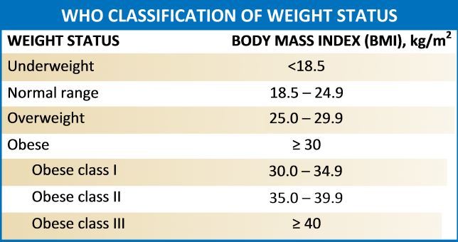
WHO Classification of BMI

Data

Our data include summaries of BMI from 200 countries worldwide, both at the national level and in urban and rural areas separately, for the years 1985 and 2017, separately for men and women. The original data source is NCD-RisC, the non-communicable disease risk factor collaboration. 2017 remains the most recent year for which they have published BMI broken out by urban/rural status.

Data Wrangling

Often we need to wrangle our data to extract meaning. This includes calculating new variables, summary statistics, grouping by variables, renaming, reordering, selecting subsets of data, filtering by various conditions, etc.

We can accomplish a great deal of wrangling by learning just seven key verbs. Each of these functions takes a data frame as input and returns a data frame as output.

• filter
• arrange
• select
• slice
• mutate
• summarize
• group_by

---

We first explore the data a bit.

load("../data/BMI_long.Rdata")
glimpse(BMI_long)

Rows: 2,400
Columns: 5
$ Country <chr> "Afghanistan", "Afghanistan", "Afghanistan", "A…
$ Sex     <chr> "Men", "Men", "Men", "Men", "Men", "Men", "Wome…
$ Region  <chr> "National", "Rural", "Urban", "National", "Rura…
$ Year    <chr> "1985", "1985", "1985", "2017", "2017", "2017",…
$ BMI     <dbl> 20.2, 19.7, 22.4, 22.8, 22.5, 23.6, 20.6, 20.1,…

names(BMI_long)

[1] "Country" "Sex"     "Region"  "Year"    "BMI"    

---

head(BMI_long)

# A tibble: 6 × 5
  Country     Sex   Region   Year    BMI
  <chr>       <chr> <chr>    <chr> <dbl>
1 Afghanistan Men   National 1985   20.2
2 Afghanistan Men   Rural    1985   19.7
3 Afghanistan Men   Urban    1985   22.4
4 Afghanistan Men   National 2017   22.8
5 Afghanistan Men   Rural    2017   22.5
6 Afghanistan Men   Urban    2017   23.6

The head() function returns “A tibble: 6 x 5” and then the first six rows of the BMI_long data. A tibble is a tweaked, opinionated version of the R data frame.

---

There are a few differences a tidyverse tibble and an R data frame. We discuss two primary differences.

First, a tibble provides more information than a data frame. When you print a tibble, it will show the first ten rows and all of the columns that fit on the screen, along with the type of each column.

You can modify the number of rows and columns shown using the print() function options.

Second, tibbles are somewhat more strict than data frames when it comes to subsetting data.

---

select()

The select() function picks off one or more columns by name.

Let’s say we want a dataset that only contains the variable BMI.

select(BMI_long, BMI)

# A tibble: 2,400 × 1
    BMI
  <dbl>
1  20.2
2  19.7
3  22.4
4  22.8
5  22.5
6  23.6
# ℹ 2,394 more rows

---

We can also use select() to exclude variables. Let’s exclude BMI but keep all other variables.

select(BMI_long, -BMI)

# A tibble: 2,400 × 4
  Country     Sex   Region   Year 
  <chr>       <chr> <chr>    <chr>
1 Afghanistan Men   National 1985 
2 Afghanistan Men   Rural    1985 
3 Afghanistan Men   Urban    1985 
4 Afghanistan Men   National 2017 
5 Afghanistan Men   Rural    2017 
6 Afghanistan Men   Urban    2017 
# ℹ 2,394 more rows

---

We can also use select() to select a range of variables. Here, we select the first three variables.

select(BMI_long, Country:Region)

# A tibble: 2,400 × 3
  Country     Sex   Region  
  <chr>       <chr> <chr>   
1 Afghanistan Men   National
2 Afghanistan Men   Rural   
3 Afghanistan Men   Urban   
4 Afghanistan Men   National
5 Afghanistan Men   Rural   
6 Afghanistan Men   Urban   
# ℹ 2,394 more rows

---

arrange()

The arrange() function orders rows (observations) in specific ways.

Let’s arrange the data by descending BMI, with large BMI values on top.

arrange(BMI_long, desc(BMI))

# A tibble: 2,400 × 5
  Country        Sex   Region   Year    BMI
  <chr>          <chr> <chr>    <chr> <dbl>
1 American Samoa Women Urban    2017   35.4
2 American Samoa Women National 2017   35.3
3 American Samoa Women Rural    2017   35  
4 Samoa          Women Urban    2017   34.7
5 American Samoa Men   Rural    2017   34.6
6 American Samoa Women Urban    1985   34.4
# ℹ 2,394 more rows

---

Or with low BMI values on top.

arrange(BMI_long, BMI)

# A tibble: 2,400 × 5
  Country     Sex   Region   Year    BMI
  <chr>       <chr> <chr>    <chr> <dbl>
1 Bangladesh  Women Rural    1985   17.7
2 Bangladesh  Women National 1985   18.2
3 Timor-Leste Women Rural    1985   18.2
4 Viet Nam    Women Rural    1985   18.2
5 Nepal       Women Rural    1985   18.3
6 Ethiopia    Men   Rural    1985   18.4
# ℹ 2,394 more rows

---

Or by two factors…

arrange(BMI_long, desc(Country), BMI)

# A tibble: 2,400 × 5
  Country  Sex   Region   Year    BMI
  <chr>    <chr> <chr>    <chr> <dbl>
1 Zimbabwe Men   Rural    1985   20.9
2 Zimbabwe Men   National 1985   21.2
3 Zimbabwe Men   Rural    2017   21.9
4 Zimbabwe Men   Urban    1985   22.1
5 Zimbabwe Men   National 2017   22.3
6 Zimbabwe Men   Urban    2017   23.3
# ℹ 2,394 more rows

---

The Pipe

The pipe is a technique for passing information from one process to another.

BMI_long %>%
  arrange(desc(BMI)) %>%
  select(Country, BMI)

# A tibble: 2,400 × 2
  Country          BMI
  <chr>          <dbl>
1 American Samoa  35.4
2 American Samoa  35.3
3 American Samoa  35  
4 Samoa           34.7
5 American Samoa  34.6
6 American Samoa  34.4
# ℹ 2,394 more rows

When reading code “in English”, say “and then” whenever you see a pipe.

---

R also has an alternative pipe, which is |> instead of %>%. Feel free to use either one.

Keyboard shortcut: command-shift-M (mac) or control-shift-M (windows)

---

slice()

Slice selects rows based on their position.

Here we slice off the first 5 rows of the BMI_long data.

BMI_long %>%
  slice(1:5)

# A tibble: 5 × 5
  Country     Sex   Region   Year    BMI
  <chr>       <chr> <chr>    <chr> <dbl>
1 Afghanistan Men   National 1985   20.2
2 Afghanistan Men   Rural    1985   19.7
3 Afghanistan Men   Urban    1985   22.4
4 Afghanistan Men   National 2017   22.8
5 Afghanistan Men   Rural    2017   22.5

---

Question: What is the code chunk below accomplishing? Guess before running the code.

BMI_long %>%
  arrange(desc(BMI)) %>%
  slice(1:5)

Click to reveal output

# A tibble: 5 × 5
  Country        Sex   Region   Year    BMI
  <chr>          <chr> <chr>    <chr> <dbl>
1 American Samoa Women Urban    2017   35.4
2 American Samoa Women National 2017   35.3
3 American Samoa Women Rural    2017   35  
4 Samoa          Women Urban    2017   34.7
5 American Samoa Men   Rural    2017   34.6

---

To add comments to code, use the pound sign. This is helpful for debugging as well - you can temporarily disable a line.

Question: What will happen if you comment out the line containing arrange() in the previous code chunk? Try it.

BMI_long %>%
  # arrange(desc(BMI)) %>%
  slice(1:5)

Click to reveal output

# A tibble: 5 × 5
  Country     Sex   Region   Year    BMI
  <chr>       <chr> <chr>    <chr> <dbl>
1 Afghanistan Men   National 1985   20.2
2 Afghanistan Men   Rural    1985   19.7
3 Afghanistan Men   Urban    1985   22.4
4 Afghanistan Men   National 2017   22.8
5 Afghanistan Men   Rural    2017   22.5

---

filter()

filter() selects rows satisfying certain conditions.

We can use a single condition. Here we select all rows where the country is Iceland.

BMI_long %>%
  filter(Country == "Iceland")

# A tibble: 12 × 5
  Country Sex   Region   Year    BMI
  <chr>   <chr> <chr>    <chr> <dbl>
1 Iceland Men   National 1985   24.8
2 Iceland Men   Rural    1985   25.2
3 Iceland Men   Urban    1985   24.8
4 Iceland Men   National 2017   27.1
5 Iceland Men   Rural    2017   27.3
6 Iceland Men   Urban    2017   27.1
# ℹ 6 more rows

---

We can use more than one condition. Here we select all rows where the Country is Iceland and the year is 2017.

BMI_long %>%
  filter(Country == "Iceland", Year == 2017)

# A tibble: 6 × 5
  Country Sex   Region   Year    BMI
  <chr>   <chr> <chr>    <chr> <dbl>
1 Iceland Men   National 2017   27.1
2 Iceland Men   Rural    2017   27.3
3 Iceland Men   Urban    2017   27.1
4 Iceland Women National 2017   25.5
5 Iceland Women Rural    2017   25.9
6 Iceland Women Urban    2017   25.5

---

More complex conditions are possible!

Question: In plain English, what is the code below accomplishing?

BMI_long %>%
  filter(Country %in% c("Iceland", "Ireland"),
         Year == 2017 | Region == "National")

# A tibble: 16 × 5
  Country Sex   Region   Year    BMI
  <chr>   <chr> <chr>    <chr> <dbl>
1 Iceland Men   National 1985   24.8
2 Iceland Men   National 2017   27.1
3 Iceland Men   Rural    2017   27.3
4 Iceland Men   Urban    2017   27.1
5 Iceland Women National 1985   24.3
6 Iceland Women National 2017   25.5
# ℹ 10 more rows

---

The table of logical operators below will be helpful as you work with filtering.

operator	definition
<	is less than?
<=	is less than or equal to?
>	is greater than?
>=	is greater than or equal to?
==	is exactly equal to?
!=	is not equal to?
x & y	is x AND y?
x \(\mid\) y	is x OR y?

---

The table of logical operators below will be helpful as you work with filtering.

operator	definition
is.na(x)	is x NA?
!is.na(x)	is x not NA?
x %in% y	is x in y?
!(x %in% y)	is x not in y?
!x	is not x?

The final operator only makes sense if x is logical (TRUE / FALSE).

R denotes missing values by NA. Missing values can cause biased or misleading results in any analysis, and it is important to understand why values are missing before drawing conclusions from data, especially if the fraction of missing values is not very small.

---

mutate()

mutate() creates a new variable. Here we categorize BMI using the WHO classification.

Here’s our code:

BMI_long %>%
  mutate(bmiclass = cut(BMI,
    breaks = c(-Inf, 18.5, 25, 30, 35, 40, Inf),
    labels = c(
      "Underweight",
      "Normal Range",
      "Overweight",
      "Obese I",
      "Obese II",
      "Obese III"
    ),
    right = FALSE #intervals [a,b)
  )) %>%
  select(BMI, bmiclass)

---

mutate()

mutate() creates a new variable. Here we categorize BMI using the WHO classification.

Here’s our output:

# A tibble: 2,400 × 2
    BMI bmiclass    
  <dbl> <fct>       
1  20.2 Normal Range
2  19.7 Normal Range
3  22.4 Normal Range
4  22.8 Normal Range
5  22.5 Normal Range
6  23.6 Normal Range
# ℹ 2,394 more rows

---

BMI_long %>%
  mutate(bmiclass = cut(
    BMI,
    breaks = c(-Inf, 18.5, 25, 30, 35, 40, Inf),
    labels = c(
      "Underweight",
      "Normal Range",
      "Overweight",
      "Obese I",
      "Obese II",
      "Obese III"
    ),
    right = FALSE
  )) %>%
  mutate(normal_range = bmiclass == "Normal Range") %>%
  print()

Click to reveal output

# A tibble: 2,400 × 7
  Country     Sex   Region   Year    BMI bmiclass    normal_range
  <chr>       <chr> <chr>    <chr> <dbl> <fct>       <lgl>       
1 Afghanistan Men   National 1985   20.2 Normal Ran… TRUE        
2 Afghanistan Men   Rural    1985   19.7 Normal Ran… TRUE        
3 Afghanistan Men   Urban    1985   22.4 Normal Ran… TRUE        
4 Afghanistan Men   National 2017   22.8 Normal Ran… TRUE        
5 Afghanistan Men   Rural    2017   22.5 Normal Ran… TRUE        
6 Afghanistan Men   Urban    2017   23.6 Normal Ran… TRUE        
# ℹ 2,394 more rows

---

Combining mutate() and ifelse()

When you need to create a simple binary flag (Yes/No, True/False) based on a threshold within a pipeline, pairing mutate() with ifelse() is the cleanest approach.

Unlike cut(), which builds complex ranges, ifelse() handles a single boundary line efficiently.

Practical Example: Overweight Flag

To create a new variable called overweight that marks individuals with a BMI of 25 or higher as "Overweight" and everyone else as "Not Overweight":

BMI_long %>%
  mutate(overweight = ifelse(BMI >= 25, "Overweight", "Not Overweight")) %>%
  select(BMI, overweight)

# A tibble: 2,400 × 2
    BMI overweight    
  <dbl> <chr>         
1  20.2 Not Overweight
2  19.7 Not Overweight
3  22.4 Not Overweight
4  22.8 Not Overweight
5  22.5 Not Overweight
6  23.6 Not Overweight
# ℹ 2,394 more rows

How the Data Transforms

BMI	BMI >= 25 Evaluation	Resulting overweight Label
22.4	FALSE	“Not Overweight”
25.0	TRUE (Inclusive)	“Overweight”
28.1	TRUE	“Overweight”
NA	NA	NA

---

summarize()

summarize calculates summary statistics. It collapses rows into summary statistics and removes columns irrelevant to the calculation. Be sure to name your columns!

BMI_long %>%
  mutate(bmiclass = cut(BMI,
    breaks = c(-Inf, 18.5, 25, 30, 35, 40, Inf),
    labels = c(
      "Underweight",
      "Normal Range",
      "Overweight",
      "Obese I",
      "Obese II",
      "Obese III"
    ),
    right = FALSE
  )) %>%
  mutate(normal_range = bmiclass == "Normal Range") %>%
  summarize(fracnormal = mean(normal_range))

Click to reveal output

# A tibble: 1 × 1
  fracnormal
       <dbl>
1         NA

---

Question: The code chunk returns an NA. What is going wrong?

BMI_long %>%
  mutate(bmiclass = cut(BMI,
    breaks = c(-Inf, 18.5, 25, 30, 35, 40, Inf),
    labels = c(
      "Underweight",
      "Normal Range",
      "Overweight",
      "Obese I",
      "Obese II",
      "Obese III"
    ),
    right = FALSE
  )) %>%
  group_by(bmiclass) %>%
  count(bmiclass) %>%
  ungroup()

Click to reveal output

# A tibble: 6 × 2
  bmiclass         n
  <fct>        <int>
1 Underweight      7
2 Normal Range  1185
3 Overweight    1091
4 Obese I         96
5 Obese II         3
6 <NA>            18

Ahh, count() is a very useful function!

---

BMI_long %>%
  count(BMI=="NA")

Click to reveal output

# A tibble: 2 × 2
  `BMI == "NA"`     n
  <lgl>         <int>
1 FALSE          2382
2 NA               18

OK great, so the problem was with the source variable. We can just drop those few NA’s when we take the mean, so that we get the mean of the observed values. In general, one would follow up on the NA values to understand why data were missing. What seems to be the issue here?

---

Let’s print all 18 variables and see if we can tell what’s going on.

BMI_long %>%
  filter(is.na(BMI)==TRUE) %>%
  print(n=18)

Investigating Missing Values

# A tibble: 18 × 5
   Country               Sex   Region Year    BMI
   <chr>                 <chr> <chr>  <chr> <dbl>
 1 Bermuda               Men   Rural  1985     NA
 2 Bermuda               Men   Rural  2017     NA
 3 Bermuda               Women Rural  1985     NA
 4 Bermuda               Women Rural  2017     NA
 5 China (Hong Kong SAR) Men   Rural  2017     NA
 6 China (Hong Kong SAR) Women Rural  2017     NA
 7 Nauru                 Men   Rural  1985     NA
 8 Nauru                 Men   Rural  2017     NA
 9 Nauru                 Women Rural  1985     NA
10 Nauru                 Women Rural  2017     NA
11 Singapore             Men   Rural  1985     NA
12 Singapore             Men   Rural  2017     NA
13 Singapore             Women Rural  1985     NA
14 Singapore             Women Rural  2017     NA
15 Tokelau               Men   Urban  1985     NA
16 Tokelau               Men   Urban  2017     NA
17 Tokelau               Women Urban  1985     NA
18 Tokelau               Women Urban  2017     NA

This makes sense! Hong Kong, Singapore, Bermuda, and Nauru do not classify any of their population as rural; Tokelau does not classify any of its population as urban.

---

Finally, let’s get the proportion of values with mean BMI in the normal range.

BMI_long %>%
  mutate(bmiclass = cut(BMI,
    breaks = c(-Inf, 18.5, 25, 30, 35, 40, Inf),
    labels = c(
      "Underweight",
      "Normal Range",
      "Overweight",
      "Obese I",
      "Obese II",
      "Obese III"
    ),
    right = FALSE
  )) %>%
  mutate(normal_range = bmiclass == "Normal Range") %>%
  summarize(fracnormal = mean(normal_range,na.rm=TRUE))

Click to reveal output

# A tibble: 1 × 1
  fracnormal
       <dbl>
1      0.497

---

group_by()

group_by() is powerful when paired with summarize to calculate summary statistics by group. Here we find the proportion of means that are in the normal range for each region. If you don’t ungroup() after you use it, there may be unforeseen consequences down the road, so this is good practice.

BMI_long %>%
  mutate(bmiclass = cut(BMI,
    breaks = c(-Inf, 18.5, 25, 30, 35, 40, Inf),
    labels = c("Underweight","Normal Range","Overweight","Obese I","Obese II","Obese III"
    ),
    right = FALSE
  )) %>%
  mutate(normal_range = bmiclass == "Normal Range") %>%
  group_by(Region) %>%
  summarize(fracnormal = mean(normal_range,na.rm=TRUE)) %>% 
  ungroup()

Click to reveal output

# A tibble: 3 × 2
  Region   fracnormal
  <chr>         <dbl>
1 National      0.506
2 Rural         0.541
3 Urban         0.446

---

We can calculate more than one summary statistic in summarize().

BMI_long %>%
  mutate(bmiclass = cut(
    BMI,
    breaks = c(-Inf, 18.5, 25, 30, 35, 40, Inf),
    labels = c(
      "Underweight",
      "Normal Range",
      "Overweight",
      "Obese I","Obese II","Obese III"
    ),
    right = FALSE
  )) %>%
  mutate(normal_range = bmiclass == "Normal Range") %>%
  group_by(Region) %>%
  summarize(
    fracnormal = mean(normal_range, na.rm = TRUE),
    max_BMI = max(BMI, na.rm = TRUE)) %>%
  ungroup()

Click to reveal output

# A tibble: 3 × 3
  Region   fracnormal max_BMI
  <chr>         <dbl>   <dbl>
1 National      0.506    35.3
2 Rural         0.541    35  
3 Urban         0.446    35.4

---

Question: What is the code chunk below doing?

BMI_long %>%
  count(Year) %>%
  mutate(prop = n / sum(n))

Click to reveal output

# A tibble: 2 × 3
  Year      n  prop
  <chr> <int> <dbl>
1 1985   1200   0.5
2 2017   1200   0.5

---

distinct()

One more nifty command is the distinct command in R, which eliminates duplicate rows.

age <- as_tibble(c(1,1,1,2,3))
age

# A tibble: 5 × 1
  value
  <dbl>
1     1
2     1
3     1
4     2
5     3

distinct(age)

# A tibble: 3 × 1
  value
  <dbl>
1     1
2     2
3     3

---

Additional Resources

• https://style.tidyverse.org/
• https://www.opencasestudies.org/ocs-bp-rural-and-urban-obesity/