Tidying Data

Introduction to Global Health Data Science

Author

Affiliation

Amy Herring

Duke University
STA/GLHLTH 198 Fall 2026

Published

September 16, 2026

We…

have data organised in a suboptimal manner for our analysis

want to reorganize the data to carry on with our analysis

This slide deck adapted from Data Science in a Box!

Data tidying

Tidy data

“Tidy datasets are easy to manipulate, model and visualise, and have a specific structure: each variable is a column, each observation is a row, and each type of observational unit is a table.”

Tidy Data, https://vita.had.co.nz/papers/tidy-data.pdf

. . .

Note: “easy to manipulate” = “straightforward to manipulate”

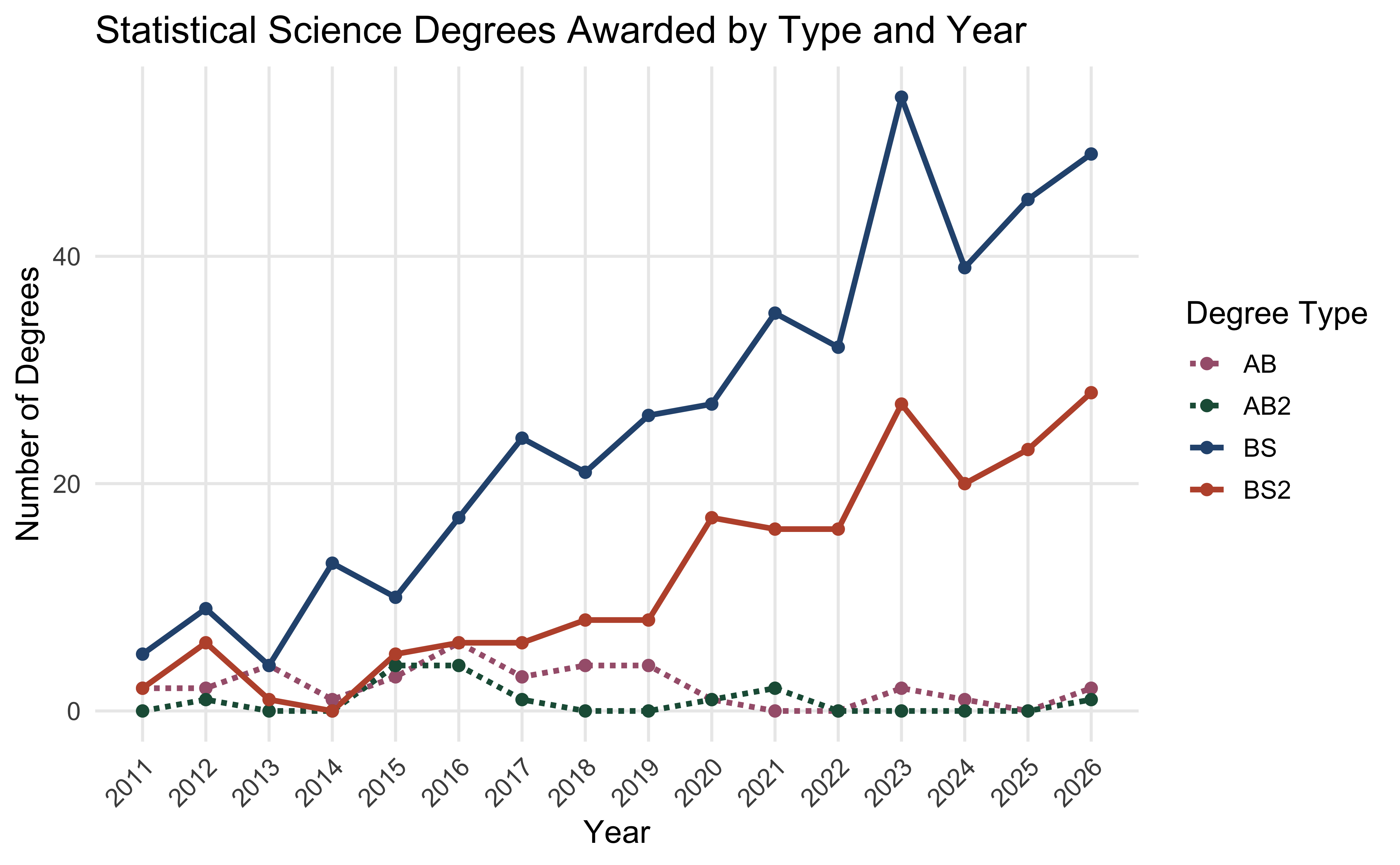
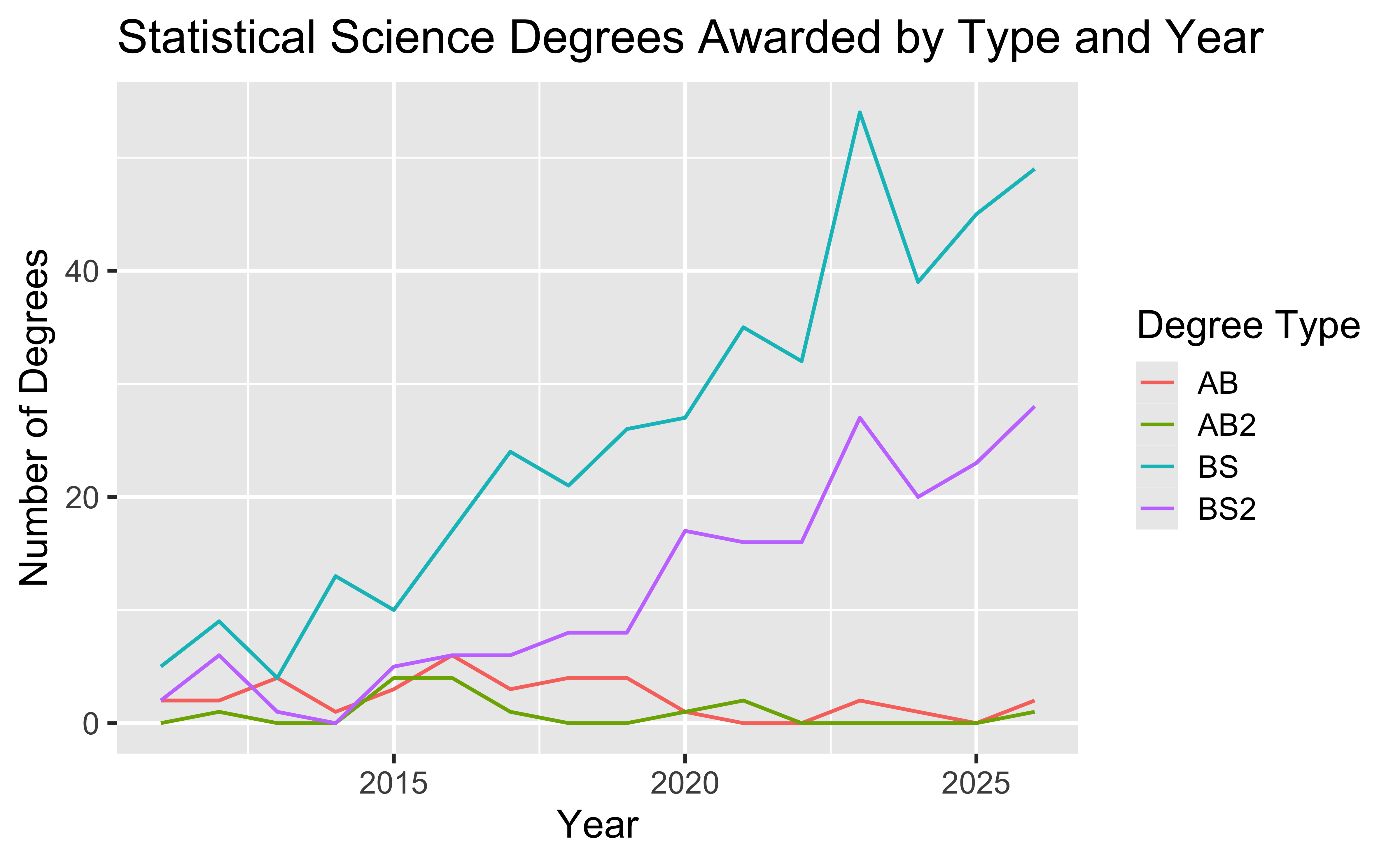
Goal: Visualize StatSci Majors Over the Years

Any ideas about the big bump in 2023?

Data

degrees

# A tibble: 4 × 17
  degree_type `2011` `2012` `2013` `2014` `2015` `2016` `2017`
  <chr>        <dbl>  <dbl>  <dbl>  <dbl>  <dbl>  <dbl>  <dbl>
1 AB               2      2      4      1      3      6      3
2 AB2              0      1      0      0      4      4      1
3 BS               5      9      4     13     10     17     24
4 BS2              2      6      1      0      5      6      6
# ℹ 9 more variables: `2018` <dbl>, `2019` <dbl>, `2020` <dbl>,
#   `2021` <dbl>, `2022` <dbl>, `2023` <dbl>, `2024` <dbl>,
#   `2025` <dbl>, `2026` <dbl>

The first column (variable) is the degree:
- AB (Bachelor of Arts)
- AB2 (Bachelor of Arts, 2nd major)
- BS (Bachelor of Science)
- BS2 (Bachelor of Science, 2nd major)
The remaining columns show the number of students graduating with that major in a given academic year from 2011 to 2026.

If you double major, your first major determines the degree you will earn. For example, if you double major in English and Statistical Science, you will graduate with a BA degree, because your first major (English) offers the BA degree. If, on the other hand, you were to make Statistical Science the first major, you would have the option to complete either the BA or the BS degree, since Statistical Science offers a BS as well as a BA track.

Let’s plan!

Review the goal plot and sketch the data frame needed to create it. What would go inside aes when we call ggplot?

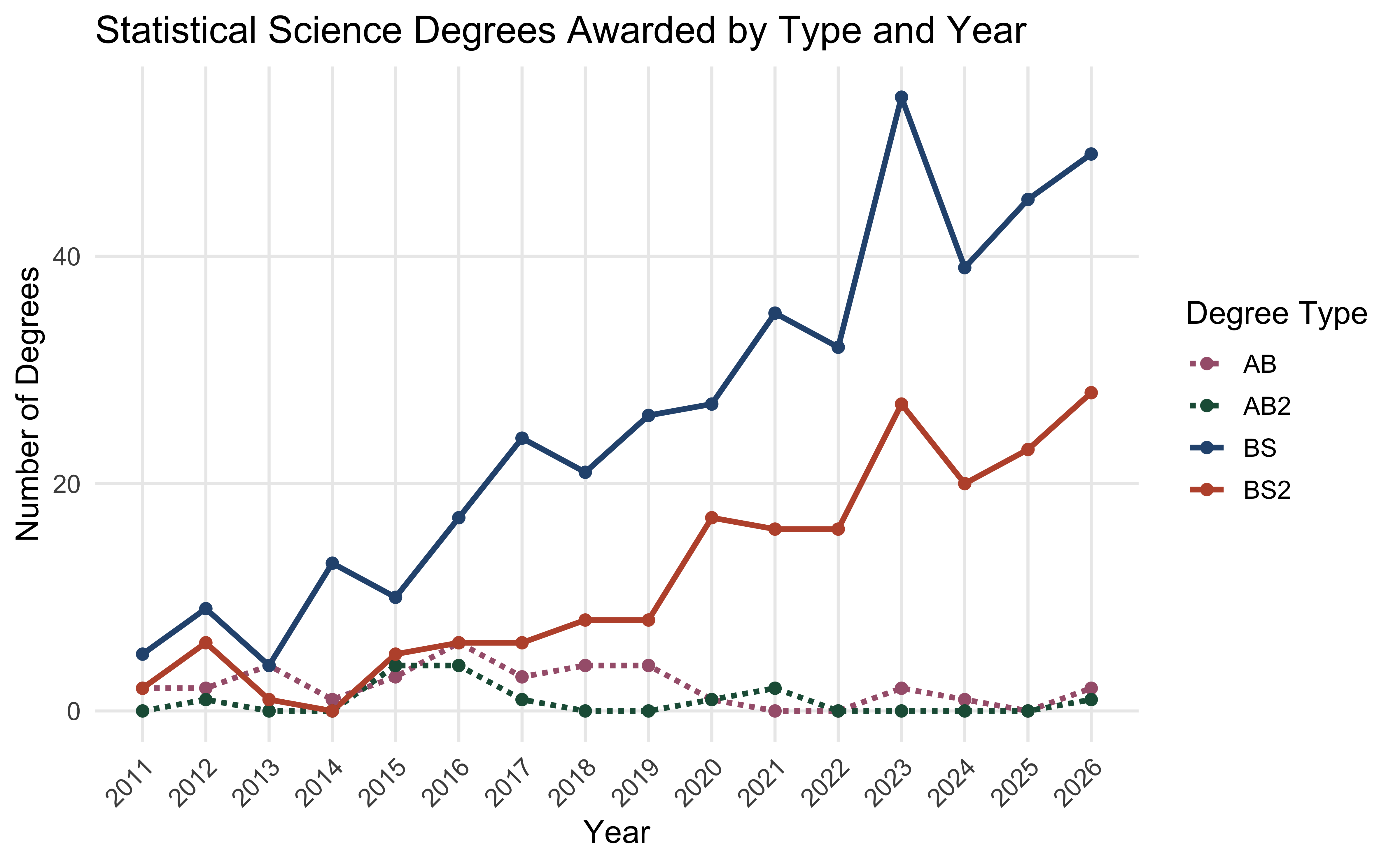
The Goal

We want to write code that starts something like this:

ggplot(degrees, aes(x = year, y = count, color = degree_type, linetype = degree_type)) + 
  ...

. . .

But our data are not in the right format :(

degrees

# A tibble: 4 × 17
  degree_type `2011` `2012` `2013` `2014` `2015` `2016` `2017`
  <chr>        <dbl>  <dbl>  <dbl>  <dbl>  <dbl>  <dbl>  <dbl>
1 AB               2      2      4      1      3      6      3
2 AB2              0      1      0      0      4      4      1
3 BS               5      9      4     13     10     17     24
4 BS2              2      6      1      0      5      6      6
# ℹ 9 more variables: `2018` <dbl>, `2019` <dbl>, `2020` <dbl>,
#   `2021` <dbl>, `2022` <dbl>, `2023` <dbl>, `2024` <dbl>,
#   `2025` <dbl>, `2026` <dbl>

We don’t even have the variables count or year.

The Challenge

How do we go from this ….

# A tibble: 4 x 16

  degree_type 2011 2012 2013 2014 2015 2016 2017 2018 2019
1          AB    2    2    4    1    3    6    3    4    4
2         AB2    0    1    0    0    4    4    1    0    0
3          BS    5    9    4   13   10   17   24   21   26
4         BS2    2    6    1    0    5    6    6    8    8

…. to this??

# A tibble: 60 x 3

   degree_type year count
1           AB 2011     2
2           AB 2012     2
3           AB 2013     4
4           AB 2014     1
5           AB 2015     3
6           AB 2016     6
7           AB 2017     3
8           AB 2018     4
9           AB 2019     4
10          AB 2020     1
11          AB 2021     0
12          AB 2022     0
13          AB 2023     2
14          AB 2024     1
15          AB 2025     0
16          AB 2026     2
17         AB2 2011     0

Pivot

`pivot_longer()`

# A tibble: 4 x 16

  degree_type 2011 2012 2013 2014 2015 2016 2017 2018 2019
1          AB    2    2    4    1    3    6    3    4    4
2         AB2    0    1    0    0    4    4    1    0    0
3          BS    5    9    4   13   10   17   24   21   26
4         BS2    2    6    1    0    5    6    6    8    8

Pivot the degrees data frame longer such that each row represents a degree type / year combination.

year and count (number of graduates for that year) are columns in the resulting data frame.

➔

# A tibble: 60 x 3

   degree_type year count
1           AB 2011     2
2           AB 2012     2
3           AB 2013     4
4           AB 2014     1
5           AB 2015     3
6           AB 2016     6
7           AB 2017     3
8           AB 2018     4
9           AB 2019     4
10          AB 2020     1
11          AB 2021     0
12          AB 2022     0
13          AB 2023     2
14          AB 2024     1
15          AB 2025     0
16          AB 2026     2
17         AB2 2011     0

`pivot_longer()`

# A tibble: 4 x 16

  degree_type 2011 2012 2013 2014 2015 2016 2017 2018 2019
1          AB    2    2    4    1    3    6    3    4    4
2         AB2    0    1    0    0    4    4    1    0    0
3          BS    5    9    4   13   10   17   24   21   26
4         BS2    2    6    1    0    5    6    6    8    8

degrees |>
  pivot_longer(
    
    cols = ___________________ ,
    
    names_to = _______________ ,
    
    values_to = ______________
  )

➔

# A tibble: 60 x 3

   degree_type year count
1           AB 2011     2
2           AB 2012     2
3           AB 2013     4
4           AB 2014     1
5           AB 2015     3
6           AB 2016     6
7           AB 2017     3
8           AB 2018     4
9           AB 2019     4
10          AB 2020     1
11          AB 2021     0
12          AB 2022     0
13          AB 2023     2
14          AB 2024     1
15          AB 2025     0
16          AB 2026     2
17         AB2 2011     0

`year`

degrees |> 
  pivot_longer(
    cols = -degree_type, # or cols = 2:16 works
    values_to = "count",
    names_to = "year"
  )

# A tibble: 64 × 3
   degree_type year  count
   <chr>       <chr> <dbl>
 1 AB          2011      2
 2 AB          2012      2
 3 AB          2013      4
 4 AB          2014      1
 5 AB          2015      3
 6 AB          2016      6
 7 AB          2017      3
 8 AB          2018      4
 9 AB          2019      4
10 AB          2020      1
# ℹ 54 more rows

What is the type of the year variable? Why? What should it be?

It’s a character (chr) variable since the information came from the columns of the original data frame.
R cannot know that these character strings represent years.
The variable type should be numeric.

`pivot_longer()` again

This time, also make sure year is a numerical variable in the resulting data frame.

degrees |>
  pivot_longer(
    cols = -degree_type,
    values_to = "count",
    names_to = "year"
  )

`pivot_longer()` again

This time, also make sure year is a numerical variable in the resulting data frame.

degrees |>
  pivot_longer(
    cols = -degree_type,
    values_to = "count",
    names_to = "year",
    names_transform = as.numeric
  )

# A tibble: 64 × 3
   degree_type  year count
   <chr>       <dbl> <dbl>
 1 AB           2011     2
 2 AB           2012     2
 3 AB           2013     4
 4 AB           2014     1
 5 AB           2015     3
 6 AB           2016     6
 7 AB           2017     3
 8 AB           2018     4
 9 AB           2019     4
10 AB           2020     1
# ℹ 54 more rows

Pivot Wider

We pivoted longer… what about wider?

# A tibble: 4 x 16

  degree_type 2011 2012 2013 2014 2015 2016 2017 2018 2019
1          AB    2    2    4    1    3    6    3    4    4
2         AB2    0    1    0    0    4    4    1    0    0
3          BS    5    9    4   13   10   17   24   21   26
4         BS2    2    6    1    0    5    6    6    8    8

Can we go the other direction?

⬅

# A tibble: 60 x 3

   degree_type year count
1           AB 2011     2
2           AB 2012     2
3           AB 2013     4
4           AB 2014     1
5           AB 2015     3
6           AB 2016     6
7           AB 2017     3
8           AB 2018     4
9           AB 2019     4
10          AB 2020     1
11          AB 2021     0
12          AB 2022     0
13          AB 2023     2
14          AB 2024     1
15          AB 2025     0
16          AB 2026     2
17         AB2 2011     0

We pivotted longer… what about wider?

# A tibble: 4 x 16

  degree_type 2011 2012 2013 2014 2015 2016 2017 2018 2019
1          AB    2    2    4    1    3    6    3    4    4
2         AB2    0    1    0    0    4    4    1    0    0
3          BS    5    9    4   13   10   17   24   21   26
4         BS2    2    6    1    0    5    6    6    8    8

degrees_long |> 
  pivot_wider(
    names_from = ____________ ,
    
    values_from = ___________ , 
  )

⬅

# A tibble: 60 x 3

   degree_type year count
1           AB 2011     2
2           AB 2012     2
3           AB 2013     4
4           AB 2014     1
5           AB 2015     3
6           AB 2016     6
7           AB 2017     3
8           AB 2018     4
9           AB 2019     4
10          AB 2020     1
11          AB 2021     0
12          AB 2022     0
13          AB 2023     2
14          AB 2024     1
15          AB 2025     0
16          AB 2026     2
17         AB2 2011     0

degrees_long |> 
  pivot_wider(
    names_from = year,
    values_from = count, 
  )

# A tibble: 4 × 17
  degree_type `2011` `2012` `2013` `2014` `2015` `2016` `2017`
  <chr>        <dbl>  <dbl>  <dbl>  <dbl>  <dbl>  <dbl>  <dbl>
1 AB               2      2      4      1      3      6      3
2 AB2              0      1      0      0      4      4      1
3 BS               5      9      4     13     10     17     24
4 BS2              2      6      1      0      5      6      6
# ℹ 9 more variables: `2018` <dbl>, `2019` <dbl>, `2020` <dbl>,
#   `2021` <dbl>, `2022` <dbl>, `2023` <dbl>, `2024` <dbl>,
#   `2025` <dbl>, `2026` <dbl>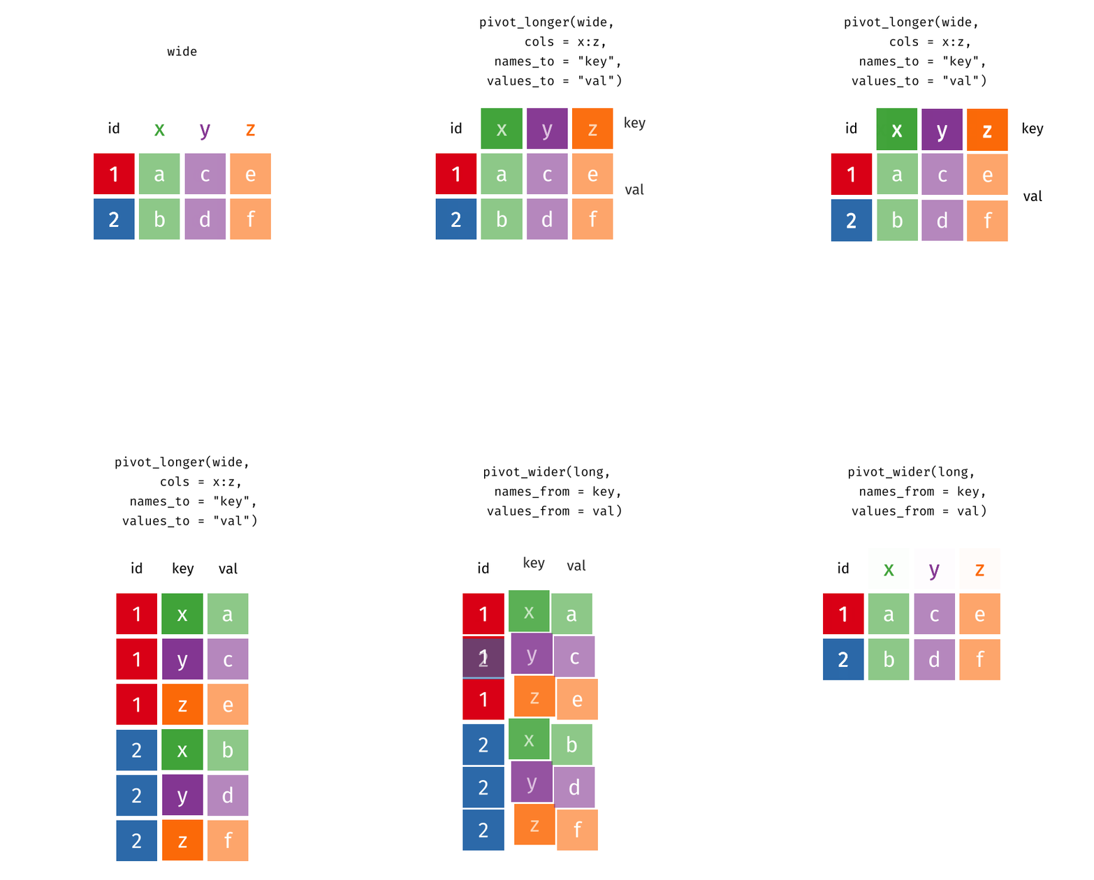

Recap: Pivot

When should you pivot? If all of the data you need is in your data frame, but the columns you need don’t exist, there is a good chance it’s time to pivot!
Wide and long: Data sets can’t be labeled as wide or long but they can be made wider or longer for a certain analysis that requires a certain format
Pivot longer - data type: When pivoting longer, variable names that turn into values are characters by default. If you need them to be in another format, you need to explicitly make that transformation, which you can do so within the pivot_longer() function.

Now for the Plot!

ggplot(degrees_long, 
       aes(x = year, y = count, color = degree_type)) +
  geom_line()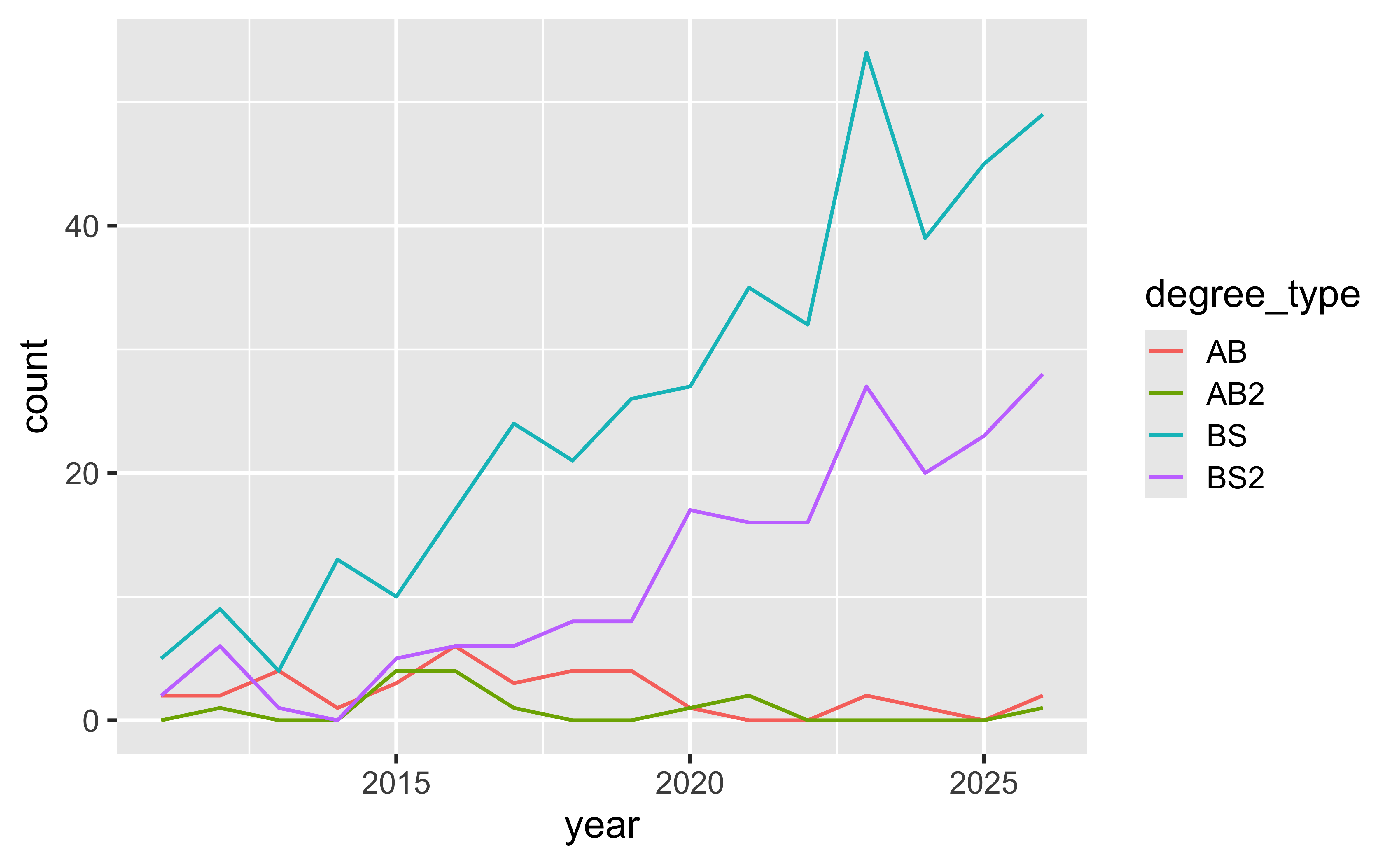

First, let’s fix the labels.

ggplot(degrees_long, 
       aes(x = year, y = count, color = degree_type)) +
  geom_line() +
  labs(
    title = "Statistical Science Degrees Awarded by Type and Year",
    x = "Year",
    y = "Number of Degrees",
    color = "Degree Type"
  )

I’d like to make it print all the year values, not just every 5th year.

ggplot(degrees_long, 
       aes(x = year, y = count, color = degree_type)) +
  geom_line() +
  labs(
    title = "Statistical Science Degrees Awarded by Type and Year",
    x = "Year",
    y = "Number of Degrees",
    color = "Degree Type"
  ) + 
  scale_x_continuous(breaks = unique(degrees_long$year))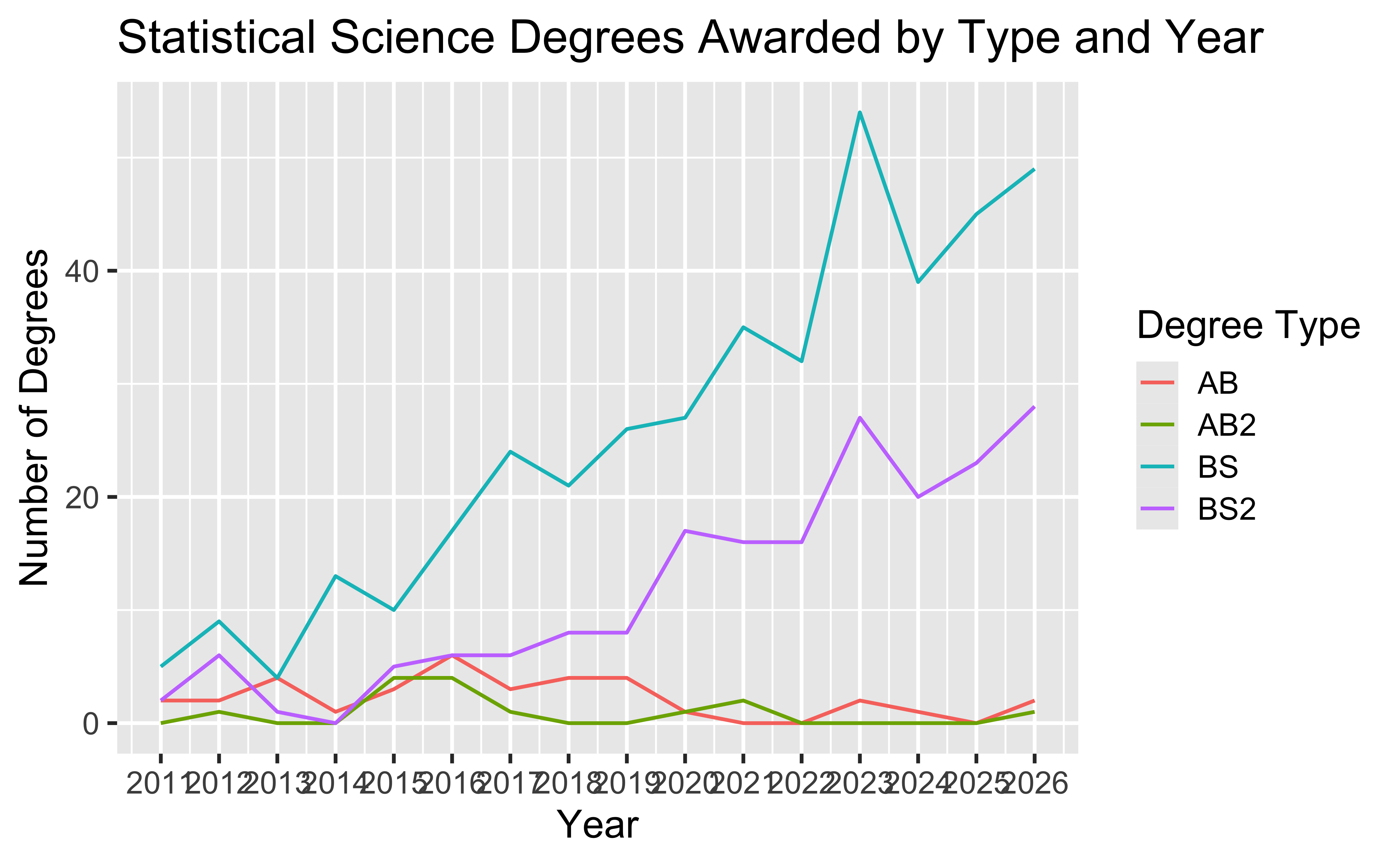

Yuck, the years print on top of each other. Let’s adjust that.

ggplot(degrees_long, 
       aes(x = year, y = count, color = degree_type)) +
  geom_line() +
  labs(
    title = "Statistical Science Degrees Awarded by Type and Year",
    x = "Year",
    y = "Number of Degrees",
    color = "Degree Type"
  ) + scale_x_continuous(breaks = unique(degrees_long$year)) +
    theme(axis.text.x = element_text(angle = 45, hjust=1))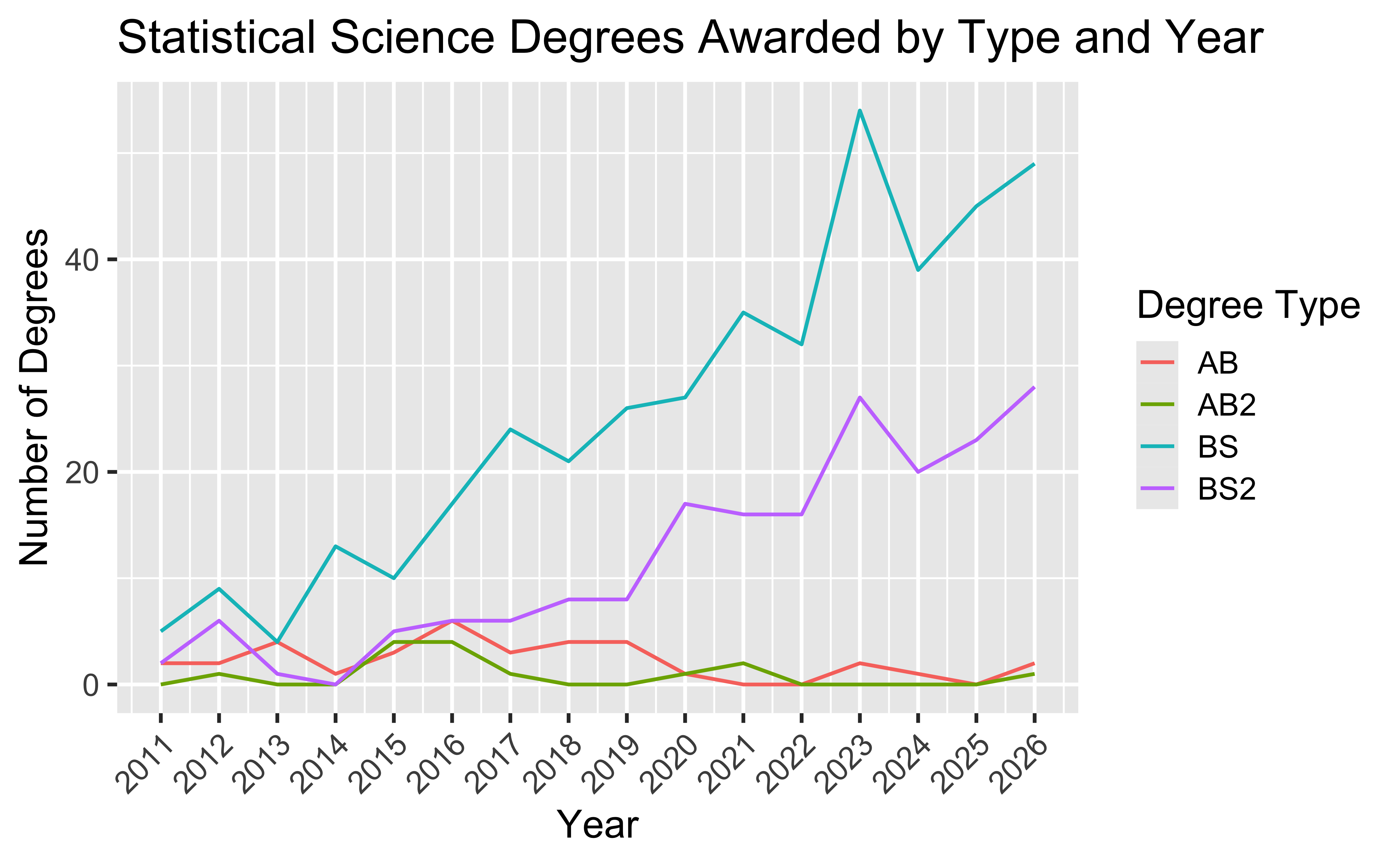

That’s pretty good. If you want to play with more bells and whistles later, the full code is here.

fall_pantone_colors <- c(
  "AB"  = "#A6617B",  # foxglove
  "AB2" = "#1E5B45",   # neptune green
  "BS"  = "#2B547E",  # regatta
  "BS2" = "#BD5338"  # autumn spice
)
line_types <- c(
  "AB"  = "11", # fine dash: 1pt on, 1pt off
  "AB2" = "11",
  "BS"  = "solid",
  "BS2" = "solid"
)
ggplot(degrees_long, aes(x = year, y = count, color = degree_type, linetype = degree_type)) +
  geom_line(linewidth = 1.1) +
  geom_point(size = 1.8) +
  scale_color_manual(values = fall_pantone_colors) +
  scale_linetype_manual(values = line_types) +
  scale_x_continuous(breaks = unique(degrees_long$year)) +
  labs(
    title = "Statistical Science Degrees Awarded by Type and Year",
    x = "Year",
    y = "Number of Degrees",
    color = "Degree Type",
    linetype = "Degree Type"
  ) +
  theme_minimal(base_size = 13) +
  theme(
    axis.text.x = element_text(angle = 45, hjust = 1),
    panel.grid.minor = element_blank(),
    legend.position = "right"
  )

We…

Data tidying

Tidy data

Goal: Visualize StatSci Majors Over the Years

Data

Let’s plan!

The Goal

The Challenge

Pivot

pivot_longer()

pivot_longer()

year

pivot_longer() again

pivot_longer() again

Pivot Wider

We pivoted longer… what about wider?

We pivotted longer… what about wider?

Recap: Pivot

Now for the Plot!

`pivot_longer()`

`pivot_longer()`

`year`

`pivot_longer()` again

`pivot_longer()` again