library(tidyverse)
library(tidymodels)
library(readr)
mercury <- readr::read_csv("../data/mercury_reg.csv")
mercury <-
  mercury %>%
  # scale() subtracts the mean and divides by the SD to make the units "standard deviations" like a z-score
  mutate(assets_sc=scale(SESassets)) %>%
  #another variable we may use later
  mutate(form_min_sc=scale(FM_buffer)) %>%
  #so I don't have to remember coding
  mutate(sex,sex_cat=ifelse(sex==1,"Male","Female")) %>%
  mutate(native,native_cat=ifelse(native==1,"Native","Non-native")) %>%
mutate(hairHg=exp(lhairHg))Model Fitting and Interpretation
Introduction to Global Health Data Science
Models with numeric explanatory variables
Mercury and Assets
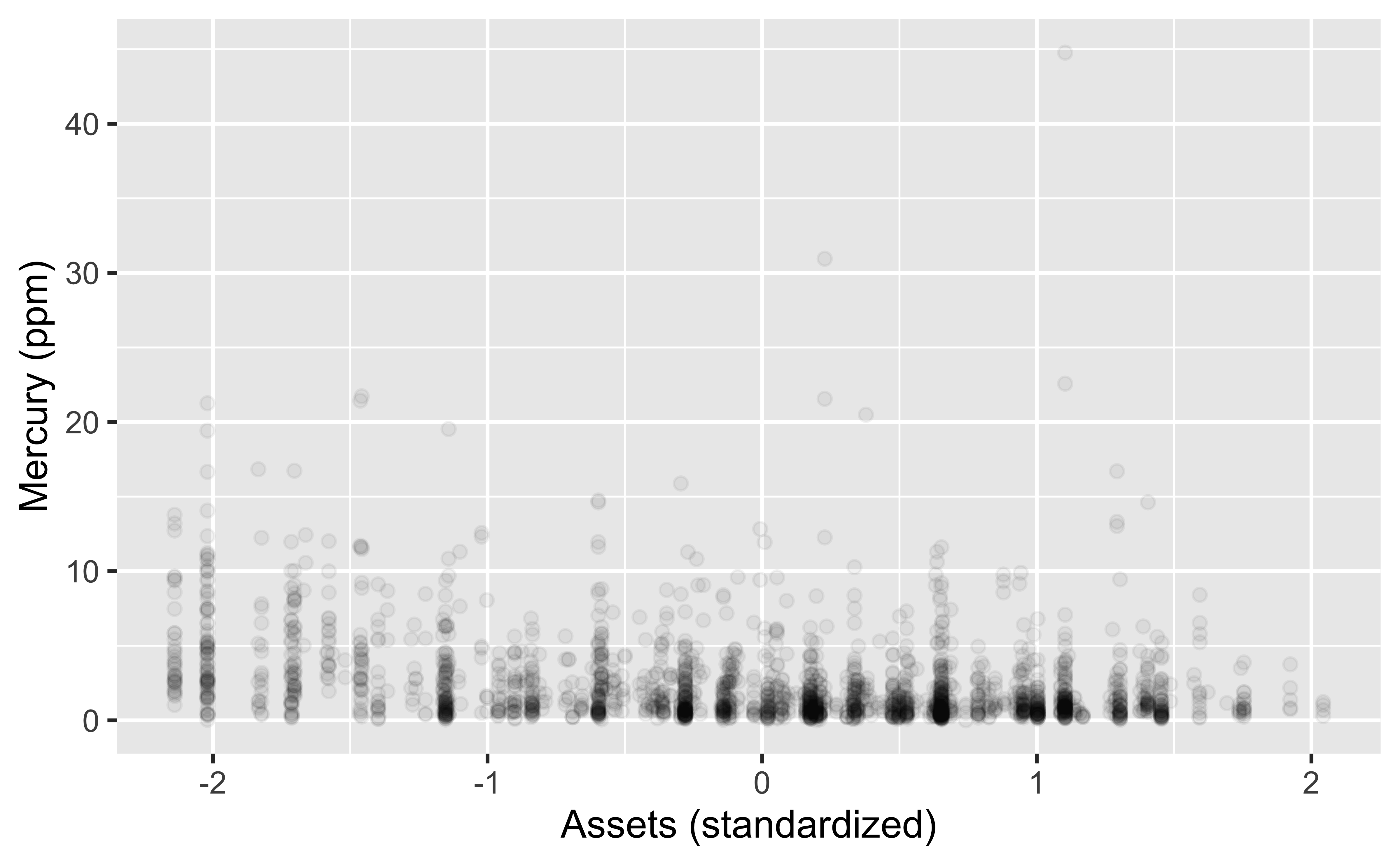
Are mercury concentrations in hair related to household socioeconomic position, as measured by assets?
Goal: Predict mercury from assets
\[\widehat{y}_{i} = \widehat{\beta}_0 + \widehat{\beta}_1 \times x_{i}\] Here \(y_i\) represents log hair mercury for subject \(i\), and \(x_i\) represents standardized household income.
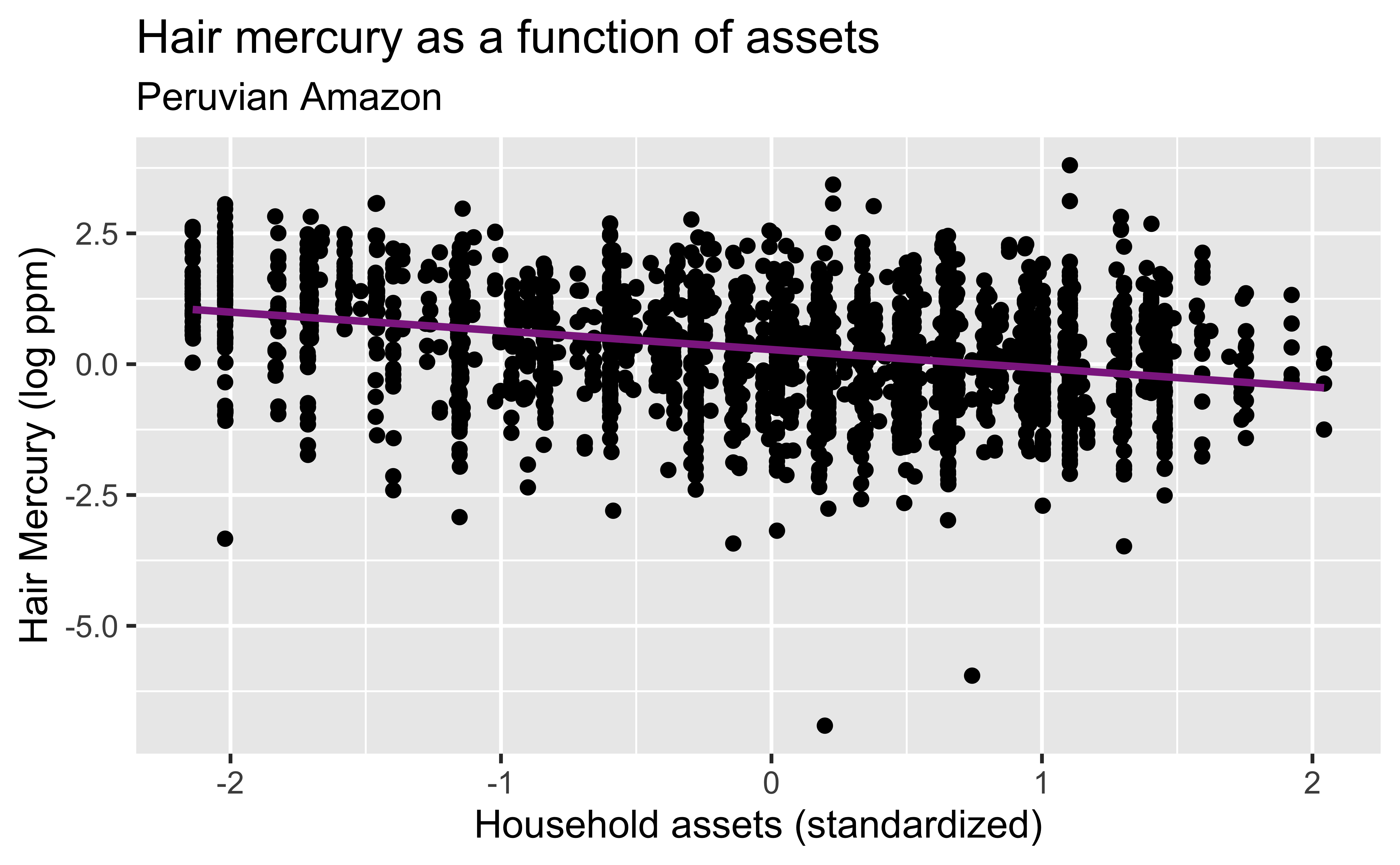
Goal: Predict mercury from assets
The model itself is given by \[y_i=\beta_0+\beta_1x_i+\varepsilon_i,\] where \(\varepsilon_i\) represents a Gaussian error term, which implies that \(y_i\) itself follows a Gaussian distribution conditional on the predictor \(x_i\).
The typical hypothesis of interest is \[H_0: \beta=0,\] which corresponds to no (linear) relationship between the predictor \(x\) and response \(y\), against the alternative \[H_0: \beta \neq 0.\]
\(t\)-test from a linear model
For the linear model
\[ y_i = \beta_0 + \beta_1 x_i + \varepsilon_i, \]
a \(t\)-test evaluates whether \(X\) is associated with \(Y\):
\[ H_0: \beta_1 = 0 \qquad \text{versus} \qquad H_A: \beta_1 \ne 0. \]
The test statistic compares the estimated coefficient with its uncertainty:
\[ t = \frac{\widehat{\beta}_1}{\operatorname{SE}(\widehat{\beta}_1)}. \]
Under \(H_0\),
\[ T \sim t_{n-p}, \] where \(p\) is the number of parameters in the mean specification of the model (here, \(p=2\) as we have \(\beta_0\) and \(\beta_1\) in the mean).
A large \(|t|\)—and correspondingly small \(p\)-value—provides evidence that \(X\) is associated with \(Y\).
Step 1: Specify model
linear_reg()#> Linear Regression Model Specification (regression)
#>
#> Computational engine: lmStep 2: Set model fitting engine
linear_reg() %>%
  set_engine("lm") # lm: linear model
#> Linear Regression Model Specification (regression)
#>
#> Computational engine: lmStep 3: Fit model & estimate parameters
… using formula syntax
A closer look at model output
#> parsnip model object
#>
#>
#> Call:
#> stats::lm(formula = lhairHg ~ assets_sc, data = data)
#>
#> Coefficients:
#> (Intercept) assets_sc
#> 0.2795 -0.3577\[\widehat{y}_{i} = 0.2795 - 0.3577 \times x_{i}\]
A tidy look at model output
linear_reg() %>%
  set_engine("lm") %>%
fit(lhairHg ~ assets_sc, data = mercury) %>%
tidy(conf.int=TRUE)#> # A tibble: 2 × 7
#> term estimate std.error statistic p.value conf.low conf.high
#> <chr> <dbl> <dbl> <dbl> <dbl> <dbl> <dbl>
#> 1 (Inte… 0.280 0.0213 13.1 7.49e-38 0.238 0.321
#> 2 asset… -0.358 0.0216 -16.5 3.90e-58 -0.400 -0.315The key quantity here is the slope for assets, which represents the relationship between household assets and hair mercury. The estimate and standard error provided in the output are used to evaluate the hypothesis \(H_0: \beta_1=0\), which states that there is no (linear) relationship between assets and mercury. The p-value for this hypothesis test is given by the p.value column for the asset row; the statistic column is calculated by dividing the estimate column entries by their standard errors. We have to do more digging to get the right degrees of freedom for the test, though.
We can also look at the 95% confidence interval for \(\beta_1\), which is given here by \((-0.40,-0.32)\) – because it does not contain the null value 0, we can say there is evidence of a relationship between assets and hair mercury.
A closer look at model output
The tidy output sweeps a few quantities under the rug, but we can tease them out using the glance function from broom instead.
fit <- linear_reg() %>%
  set_engine("lm") %>%
  fit(lhairHg ~ assets_sc, data = mercury)
fit %>% tidy(conf.int=TRUE)
#> # A tibble: 2 × 7
#> term estimate std.error statistic p.value conf.low conf.high
#> <chr> <dbl> <dbl> <dbl> <dbl> <dbl> <dbl>
#> 1 (Inte… 0.280 0.0213 13.1 7.49e-38 0.238 0.321
#> 2 asset… -0.358 0.0216 -16.5 3.90e-58 -0.400 -0.315#> # A tibble: 1 × 12
#> r.squared adj.r.squared sigma statistic p.value df logLik
#> <dbl> <dbl> <dbl> <dbl> <dbl> <dbl> <dbl>
#> 1 0.106 0.106 1.02 274. 3.90e-58 1 -3316.
#> AIC BIC deviance df.residual nobs
#> <dbl> <dbl> <dbl> <int> <int>
#> 1 6638. 6655. 2407. 2298 2300Here we see the \(df=n-p\) for the t-test in the df.residual column. nobs contains the number of observations used in model fitting.
Note a different statistic is presented here – it is the square of the statistic from tidy (there was some rounding). If you take a regression course, you will learn this statistic, the square of the t-statistic, follows an \(F\) distribution, which is widely used in linear models.
Slope and intercept
\[\widehat{y}_{i} = 0.280 - 0.358 \times x_{i}\]
-
Slope: For each standard deviation increase in assets, the log hair mercury level is expected to be lower, on average, by 0.358 log ppm.
- perhaps not a very useful statement given the scale
-
Intercept: Individuals with household assets at the mean level (
assets_sc=0) are expected to have hair mercury concentrations of 0.280 log ppm, on average- Remember
assets_scwas standardized, soassets_sc=0 does not mean “no assets” but instead means “average assets” as it corresponds to an assets z-score of 0.
- Remember
Slope and intercept: easy/standard case
Interpretation is a little easier without a log transformation. Suppose our outcome \(y\) is exam score, and the predictor \(x\) is hours studied, and we fit a linear model and get the following estimated line.
\[\widehat{y}_{i} = 60 + 5 \times x_{i}\]
Slope: For each additional hour of study, the exam score is expected to be higher, on average, by 5 points.
Intercept: Individuals who do not study are expected to have exam scores of 60 points, on average
Note: now you can see the danger of extrapolating beyond the range of the data. We don’t expect someone who studies 20 hours to have an exam score of 160 on a 100-point scale – at some point, mastery (hopefully not futility!) is reached.
Better Interpretation in Models with Log Transformation
Working with logs
Subtraction and logs: \(log(a) − log(b) = log(a / b)\)
Natural logarithm: \(e^{log(x)} = x\)
We can use these identities to “undo” the log transformation
Interpreting the slope
The slope coefficient for the log transformed model is -0.3577, meaning the log mercury difference between people whose household incomes are one SD apart is predicted to be -0.3577 (95% CI=(-0.400,-0.315)) log ppm.
Using this information, and properties of logs that we just reviewed, fill in the blanks in the following alternate interpretation of the slope:
For each additional SD the household assets are greater, the hair mercury concentration is expected to be
___, on average, by a factor of___.
For each additional increase in scaled assets, hair mercury content is expected to be
___, on average, by a factor of___.
\[ \log(\text{hair Hg for assets x+1}) - \log(\text{hair Hg for assets x}) = -0.3577 \]
\[ \log\left(\frac{\text{hair Hg for assets x+1}}{\text{hair Hg for assets x}}\right) = -0.3577 \]
\[ e^{\log\left(\frac{\text{Hg for assets x+1}}{\text{Hg for assets x}}\right)} = e^{-0.3577} \]
\[ \frac{\text{Hg for assets x+1}}{\text{Hg for assets x}} \approx 0.70 \]
For each SD increase in assets, the hair Hg is expected to be lower, on average, by a factor of 0.70.
You said I didn’t need a calculator!
Yup, R can do this for you!
fit <- linear_reg() %>%
  set_engine("lm") %>%
  fit(lhairHg ~ assets_sc, data = mercury)
fit %>% tidy(exponentiate=TRUE, conf.int=TRUE)
#> # A tibble: 2 × 7
#> term estimate std.error statistic p.value conf.low conf.high
#> <chr> <dbl> <dbl> <dbl> <dbl> <dbl> <dbl>
#> 1 (Inte… 1.32 0.0213 13.1 7.49e-38 1.27 1.38
#> 2 asset… 0.699 0.0216 -16.5 3.90e-58 0.670 0.730For each SD increase in assets, the hair Hg is expected to be lower, on average, by a factor of 0.70 (95% CI=(0.67, 0.73)).
Correlation does not imply causation
Remember this when interpreting model coefficients

Source: XKCD, Cell phones
Parameter estimation
Linear model with a single predictor
- We’re interested in \(\beta_0\) (population parameter for the intercept) and \(\beta_1\) (population parameter for the slope) in the following model:
\[y_{i} = \beta_0 + \beta_1~x_{i}+\varepsilon_i\]
where \(\varepsilon\) represents random error around our mean
- Tough luck, you can’t have them…
- So we use sample statistics to estimate them, using the notation \(b\) or \(\widehat{\beta}\) to distinguish our estimates from the true parameters \(\beta\)
\[\widehat{y}_{i} = b_0 + b_1~x_{i}\] or \[\widehat{y}_i = \widehat{\beta}_0 + \widehat{\beta}_1~x_i\]
Least squares regression
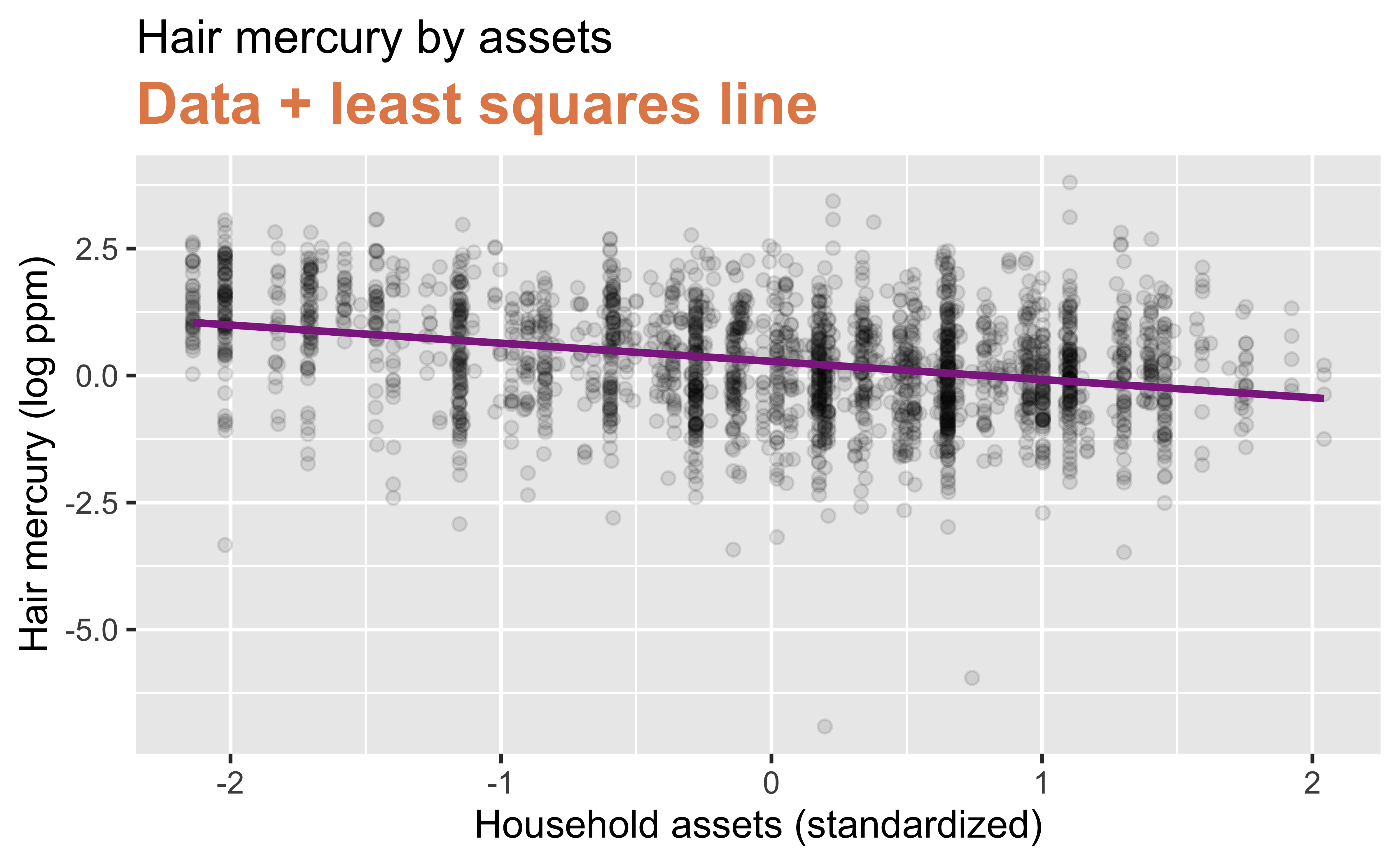
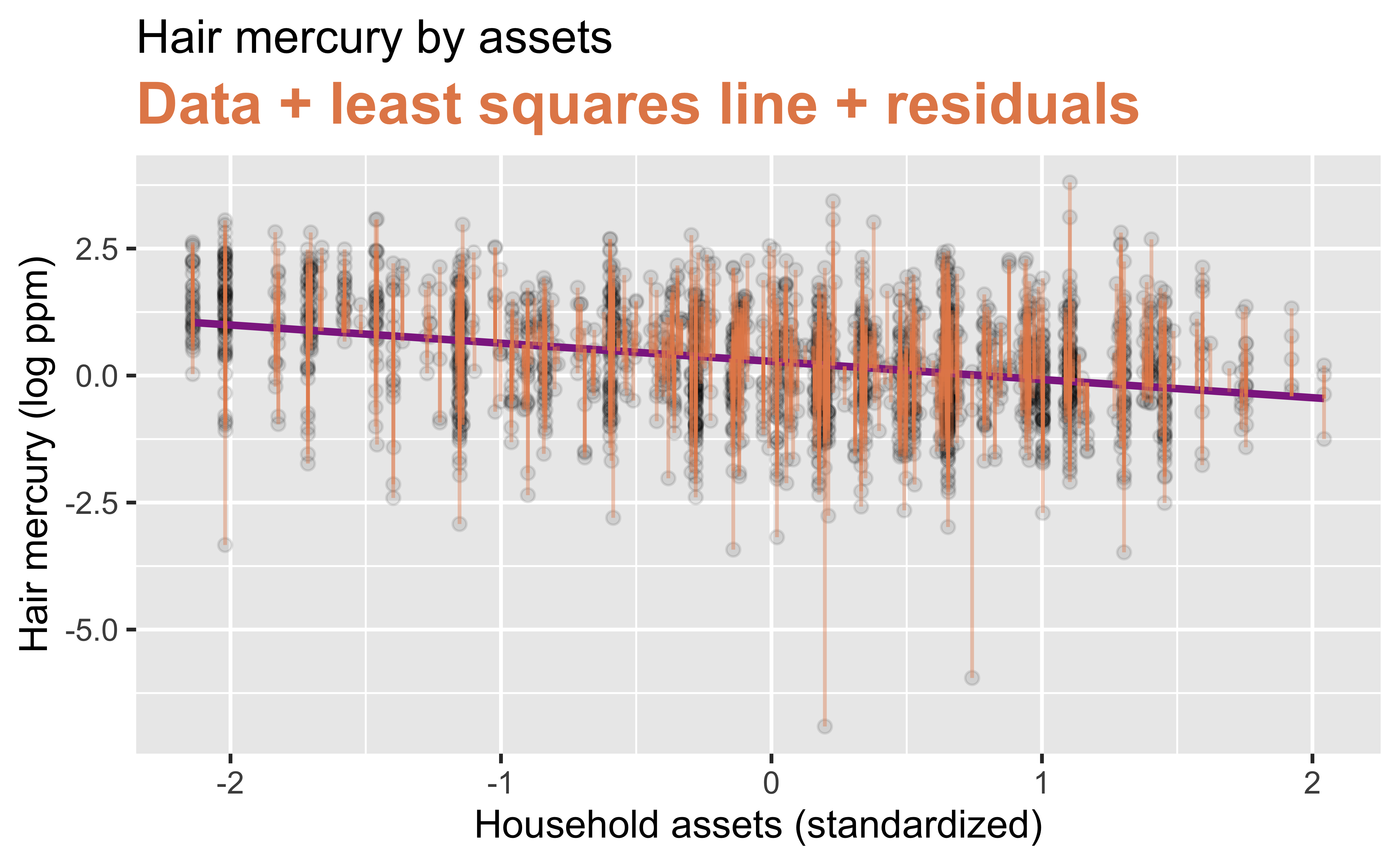
The regression line minimizes the sum of squared residuals (the residuals are estimates of the error \(\varepsilon_i\)).
If \(e_i = y_i - \hat{y}_i\), then, the regression line minimizes \(\sum_{i = 1}^n e_i^2\).
Why do we square the residuals?
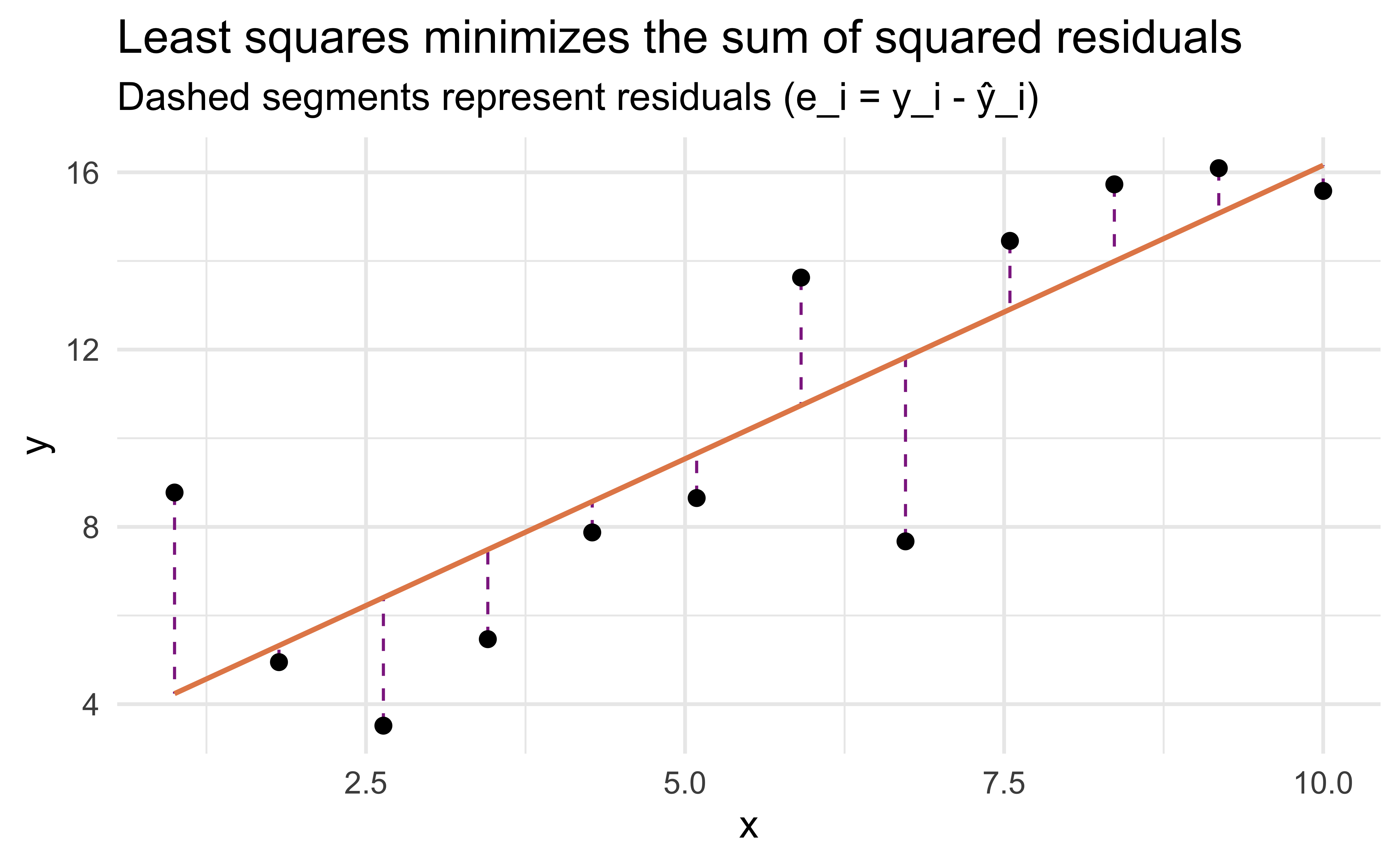
Visualizing residuals
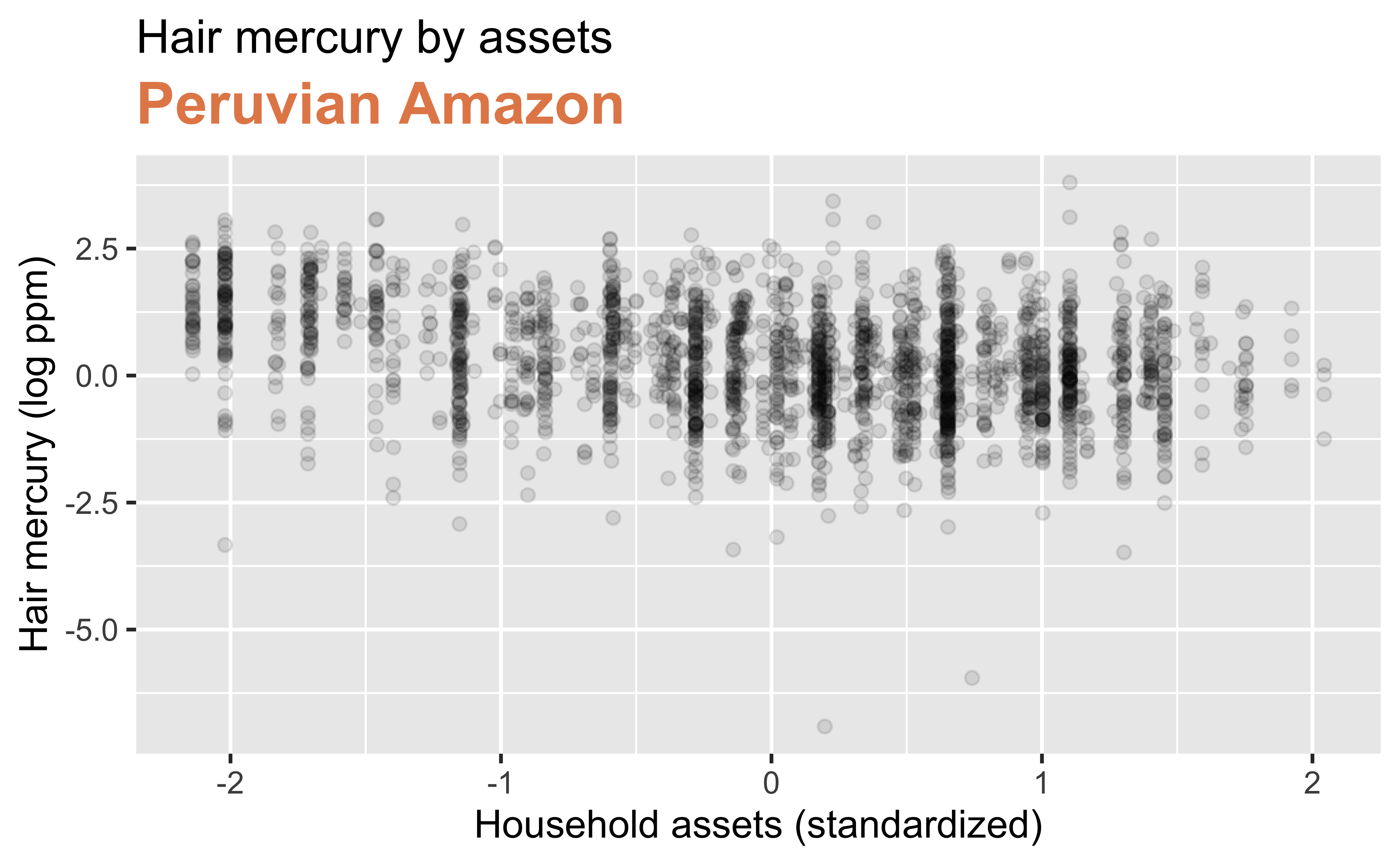
Visualizing residuals (cont.)
Visualizing residuals (cont.)
How well does the model fit? \(R^2\)
The coefficient of determination, \(R^2\), measures the proportion of variation in the response \(y\) that is explained by the regression model.
\[ R^2 = 1 - \frac{\sum_{i=1}^n (y_i-\widehat{y}_i)^2} {\sum_{i=1}^n (y_i-\bar{y})^2} \]
- \(\sum (y_i-\widehat{y}_i)^2\): variation not explained by the model
- \(\sum (y_i-\bar{y})^2\): total variation in \(y\)
\(R^2\) ranges from 0 to 1.
- \(R^2 = 0\): the model explains none of the variation in \(y\)
- \(R^2 = 1\): the model explains all of the variation in \(y\)
For simple linear regression with one predictor:
\[ R^2 = r^2 \]
We can get \(R^2\) from the glance function.
fit <- linear_reg() %>%
  set_engine("lm") %>%
  fit(lhairHg ~ assets_sc, data = mercury)
fit %>% glance() %>% print(width = Inf)
#> # A tibble: 1 × 12
#> r.squared adj.r.squared sigma statistic p.value df logLik
#> <dbl> <dbl> <dbl> <dbl> <dbl> <dbl> <dbl>
#> 1 0.106 0.106 1.02 274. 3.90e-58 1 -3316.
#> AIC BIC deviance df.residual nobs
#> <dbl> <dbl> <dbl> <int> <int>
#> 1 6638. 6655. 2407. 2298 2300While \(R^2=0.106\) may seem quite low (the corresponding estimated correlation between \(x\) and \(y\) is \(\sqrt{0.106}=0.33\)), it’s actually not too alarming given that we have observational data from humans with highly variable activities and exposures.
Properties of least squares regression
- The regression line goes through the center of mass point, the coordinates corresponding to average \(x\) and average \(y\), \((\bar{x}, \bar{y})\):
\[\bar{y} = \hat{\beta}_0 + \hat{\beta}_1 \bar{x} ~ \rightarrow ~ \hat{\beta}_0 = \bar{y} - \hat{\beta}_1 \bar{x}\]
- The slope has the same sign as the correlation coefficient: \(\hat{\beta}_1 = r \frac{s_y}{s_x}\)
- \(s_x\) is the standard deviation of the explanatory variable \(x\), and \(s_y\) is the standard deviation of the response variable \(y\)
- If \(y\) varies a lot more than \(x\) does (large \(s_y\) relative to \(s_x\)), the slope will be steeper for the same correlation — a small change in \(x\) corresponds to a much bigger typical change in \(y\)
- In our example, \(s_x\) is the standard deviation of
assets_sc(which is 1, since it was standardized), and \(s_y\) is the standard deviation oflhairHg
- The sum of the residuals is zero: \(\sum_{i = 1}^n e_i = 0\)
- The residuals and \(x\) values are uncorrelated
Model checking
“Linear” models
- We’re fitting a “linear” model, which assumes a linear relationship between our explanatory and response variables.
- But how do we assess this?
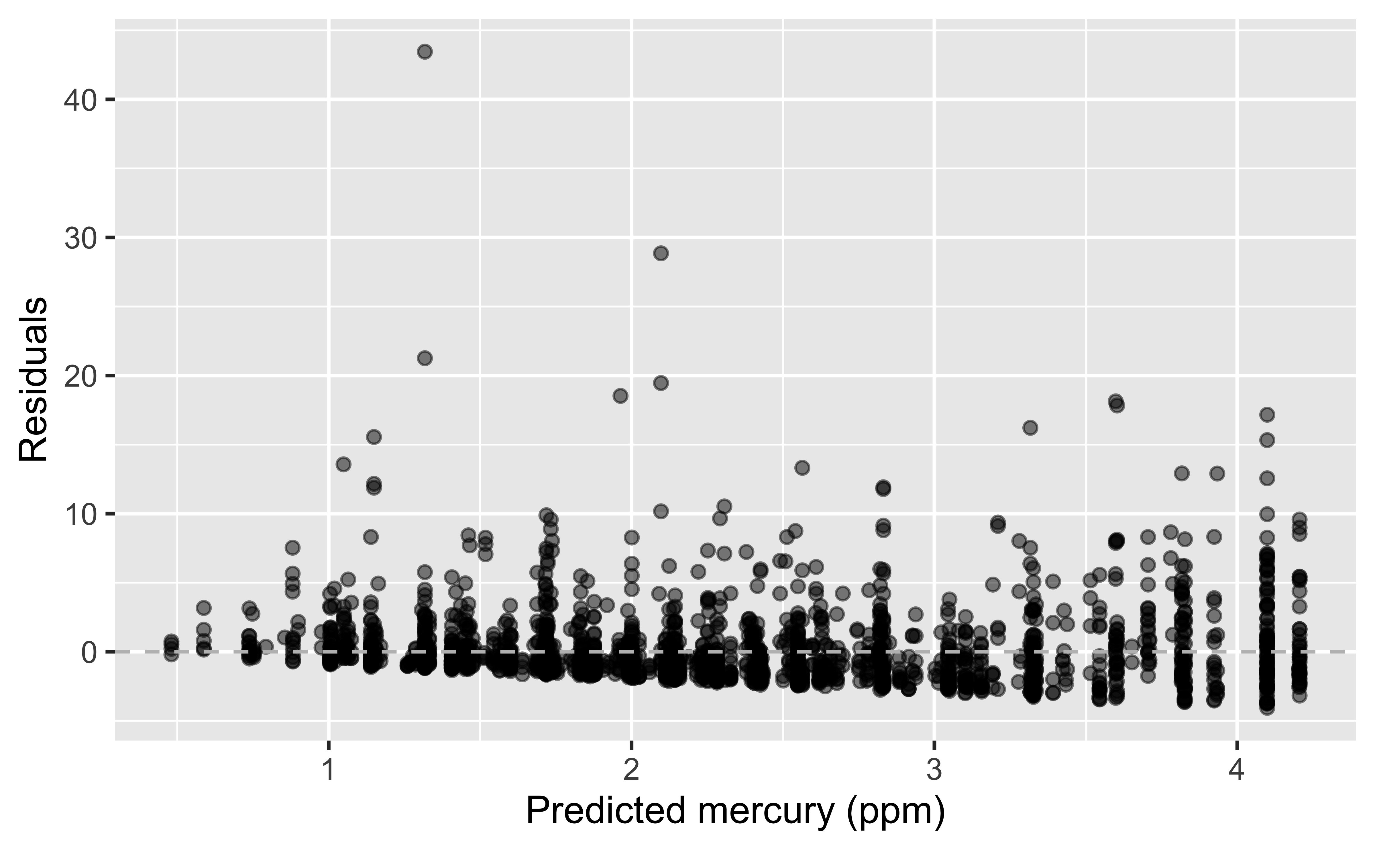
Graphical diagnostic: residuals plot (ppm units)
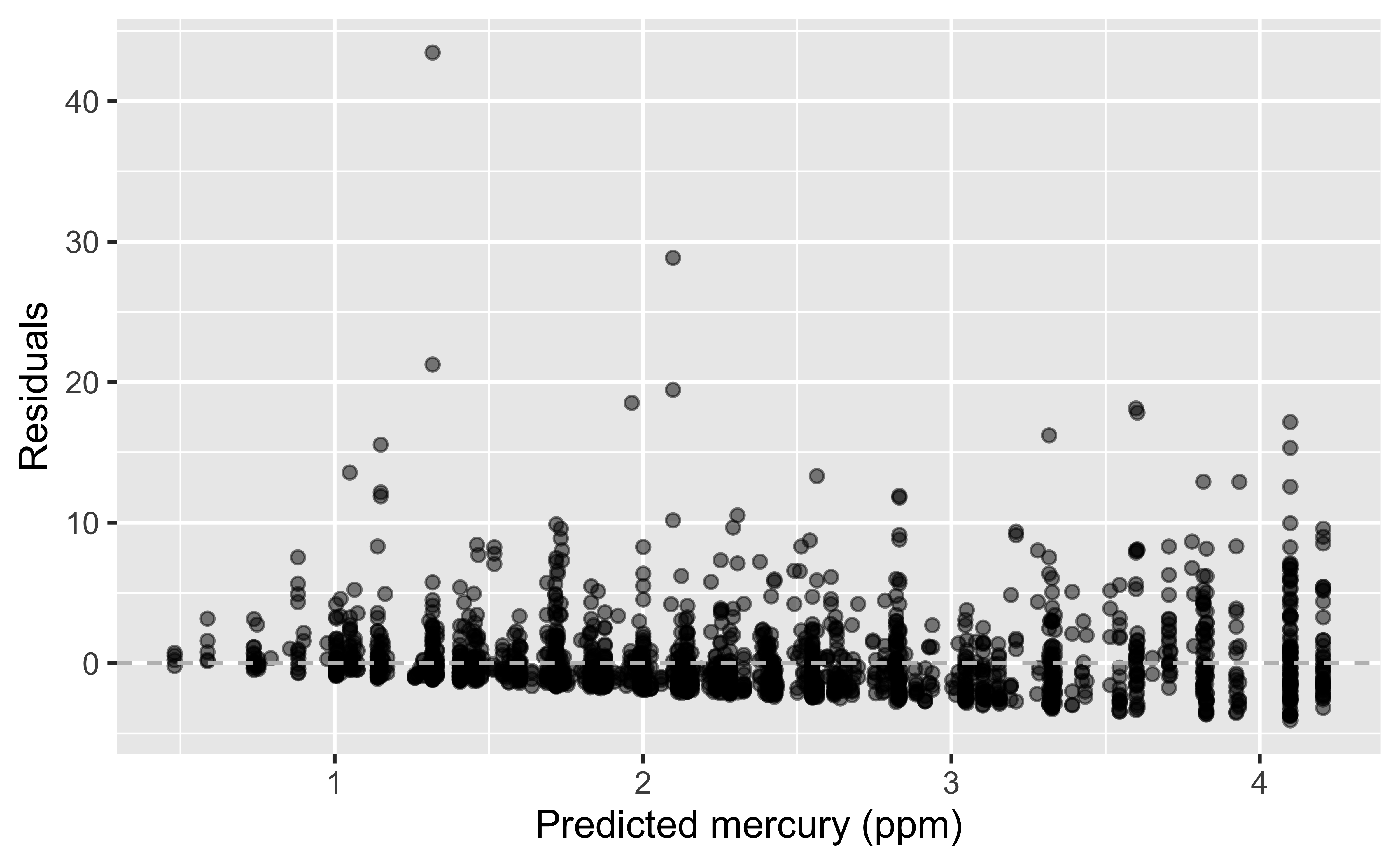
hg_asset_fit <- linear_reg() %>%
  set_engine("lm") %>%
  fit(hairHg ~ assets_sc, data = mercury)
hg_asset_fit_aug <- augment(hg_asset_fit$fit)
ggplot(hg_asset_fit_aug, mapping = aes(x = .fitted, y = .resid)) +
  geom_point(alpha = 0.5) +
  geom_hline(yintercept = 0, color = "gray", lty = "dashed") +
labs(x = "Predicted mercury (ppm)", y = "Residuals")hg_asset_fit_aug#> # A tibble: 2,300 × 9
#> .rownames hairHg assets_sc[,1] .fitted .resid .hat .sigma
#> <chr> <dbl> <dbl> <dbl> <dbl> <dbl> <dbl>
#> 1 1 1.97 -0.837 3.05 -1.08 0.000750 2.77
#> 2 3 1.10 0.197 2.12 -1.03 0.000452 2.77
#> 3 11 5.34 -0.280 2.55 2.79 0.000471 2.77
#> 4 13 1.57 -0.280 2.55 -0.981 0.000471 2.77
#> 5 14 2.02 -0.280 2.55 -0.528 0.000471 2.77
#> 6 15 0.599 -0.280 2.55 -1.95 0.000471 2.77
#> # ℹ 2,294 more rows
#> # ℹ 2 more variables: .cooksd <dbl>, .std.resid <dbl>More on augment()
glimpse(hg_asset_fit_aug)#> Rows: 2,300
#> Columns: 9
#> $ .rownames <chr> "1", "3", "11", "13", "14", "15", "16", "17"…
#> $ hairHg <dbl> 1.9652, 1.0951, 5.3366, 1.5683, 2.0218, 0.59…
#> $ assets_sc <dbl[,1]> <matrix[21 x 1]>
#> $ .fitted <dbl> 3.045165, 2.124332, 2.549503, 2.549503, …
#> $ .resid <dbl> -1.0799648, -1.0292319, 2.7870974, -0.981202…
#> $ .hat <dbl> 0.0007495801, 0.0004516563, 0.0004705556, 0.…
#> $ .sigma <dbl> 2.769771, 2.769779, 2.769252, 2.769787, 2.76…
#> $ .cooksd <dbl> 5.708620e-05, 3.122263e-05, 2.385430e-04, 2.…
#> $ .std.resid <dbl> -0.3901294, -0.3717471, 1.0066782, -0.354402…Looking for…
- Residuals distributed randomly around 0
- With no visible pattern along the x or y axes
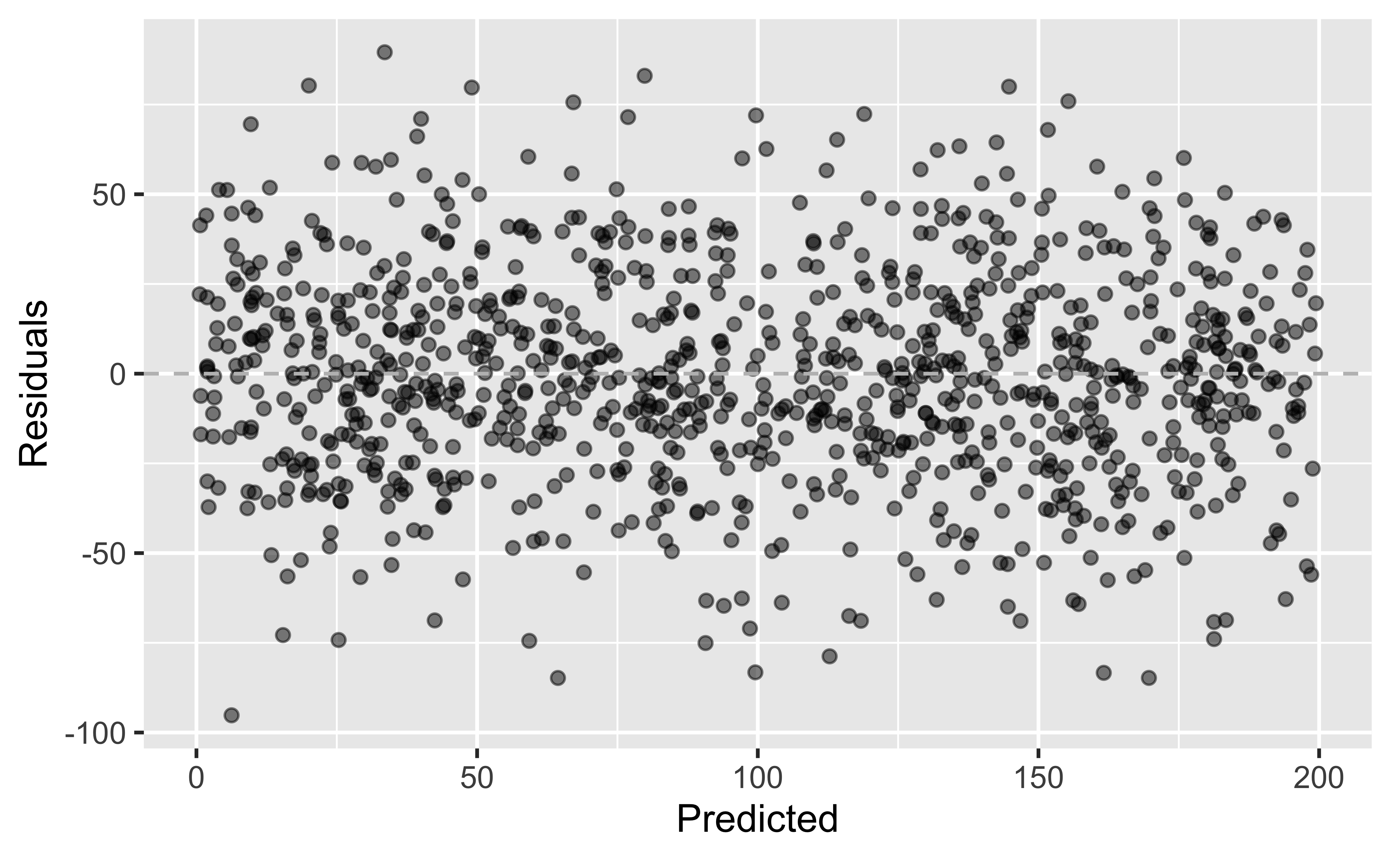
Not hoping for…
Fan shapes
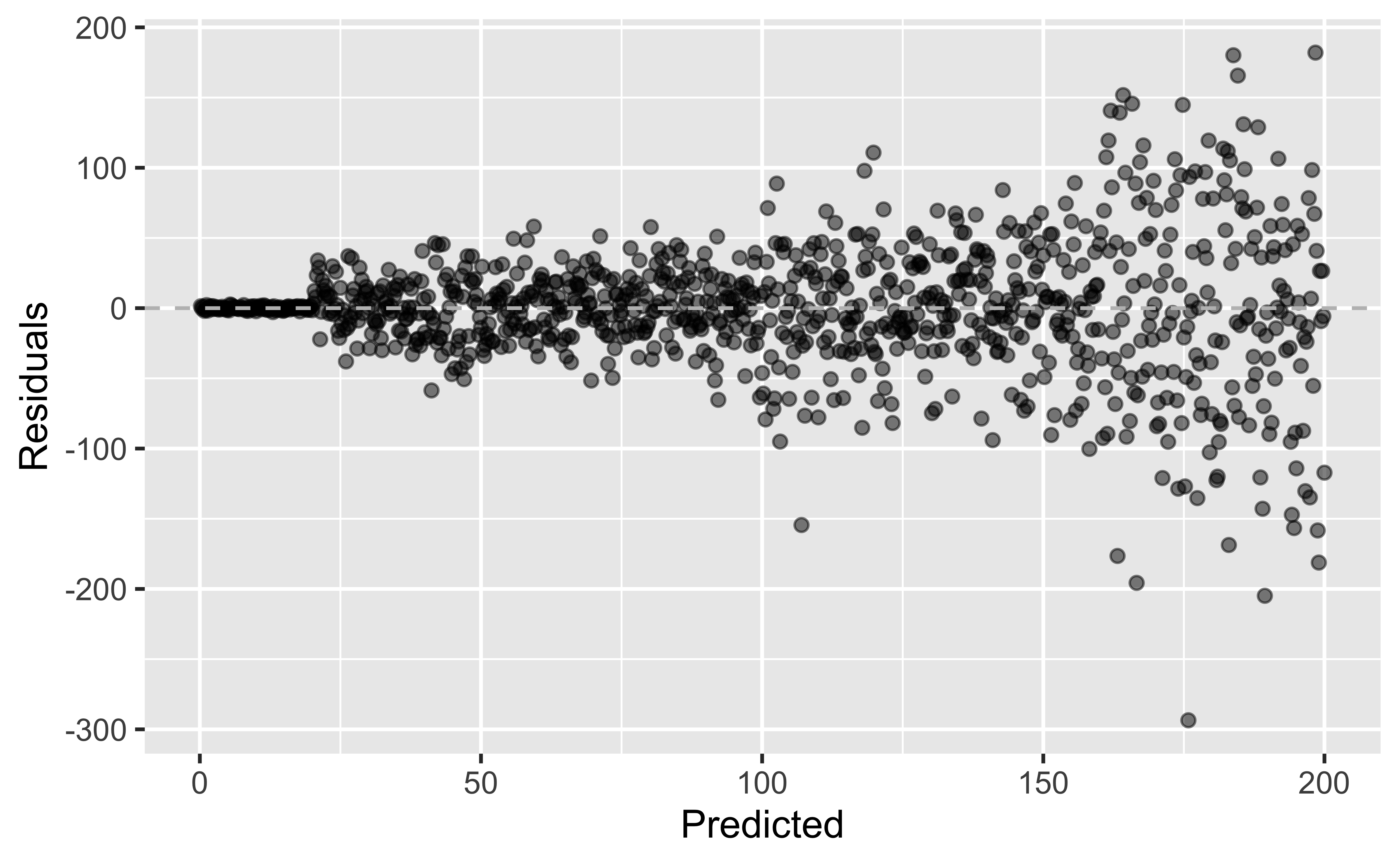
(Evidence of non-constant variance in residuals across the range of predicted values)
Not looking for…
Groups of patterns
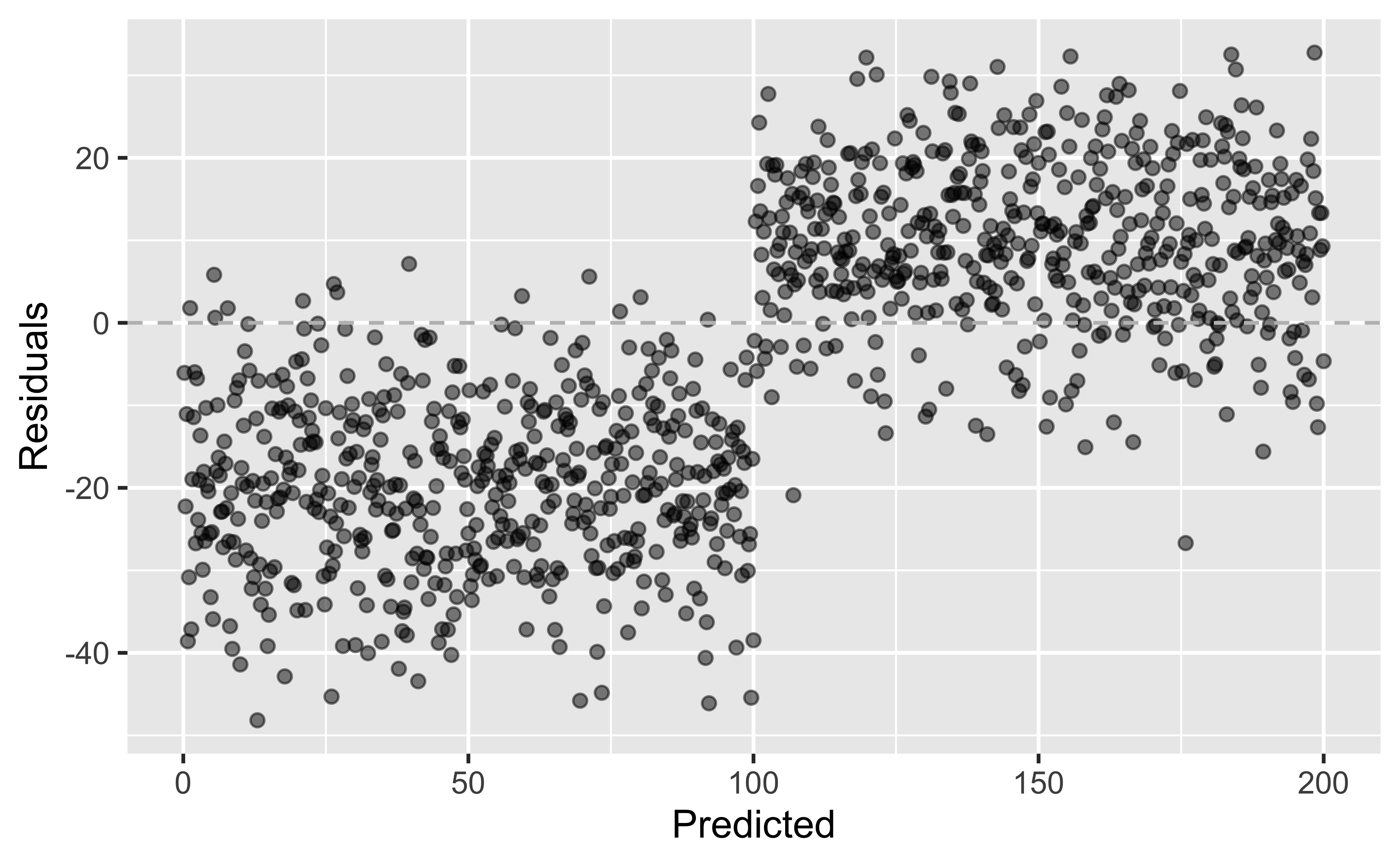
(Evidence of a missing predictor)
Not looking for…
Other non-random structure
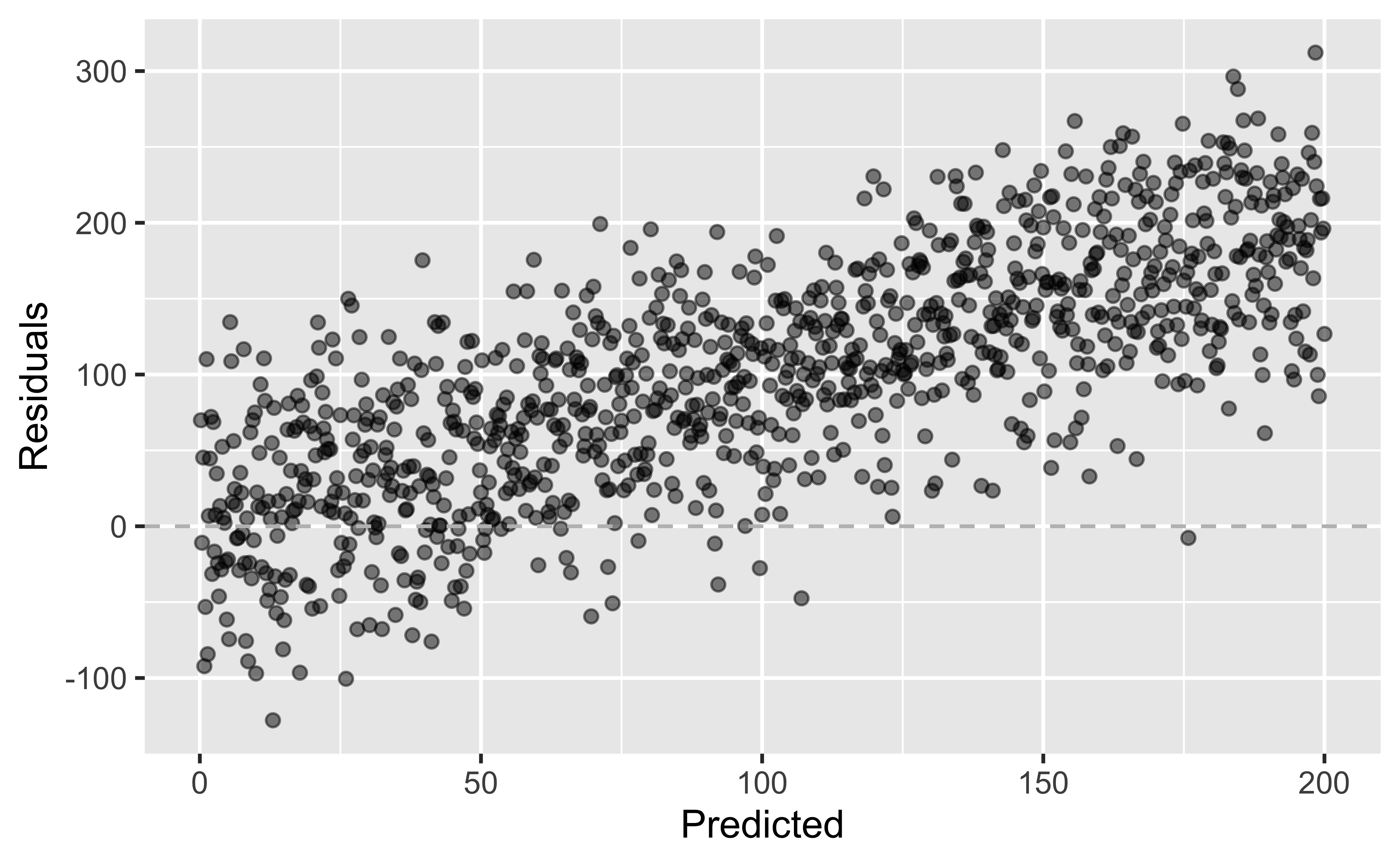
Not looking for…
Any patterns!
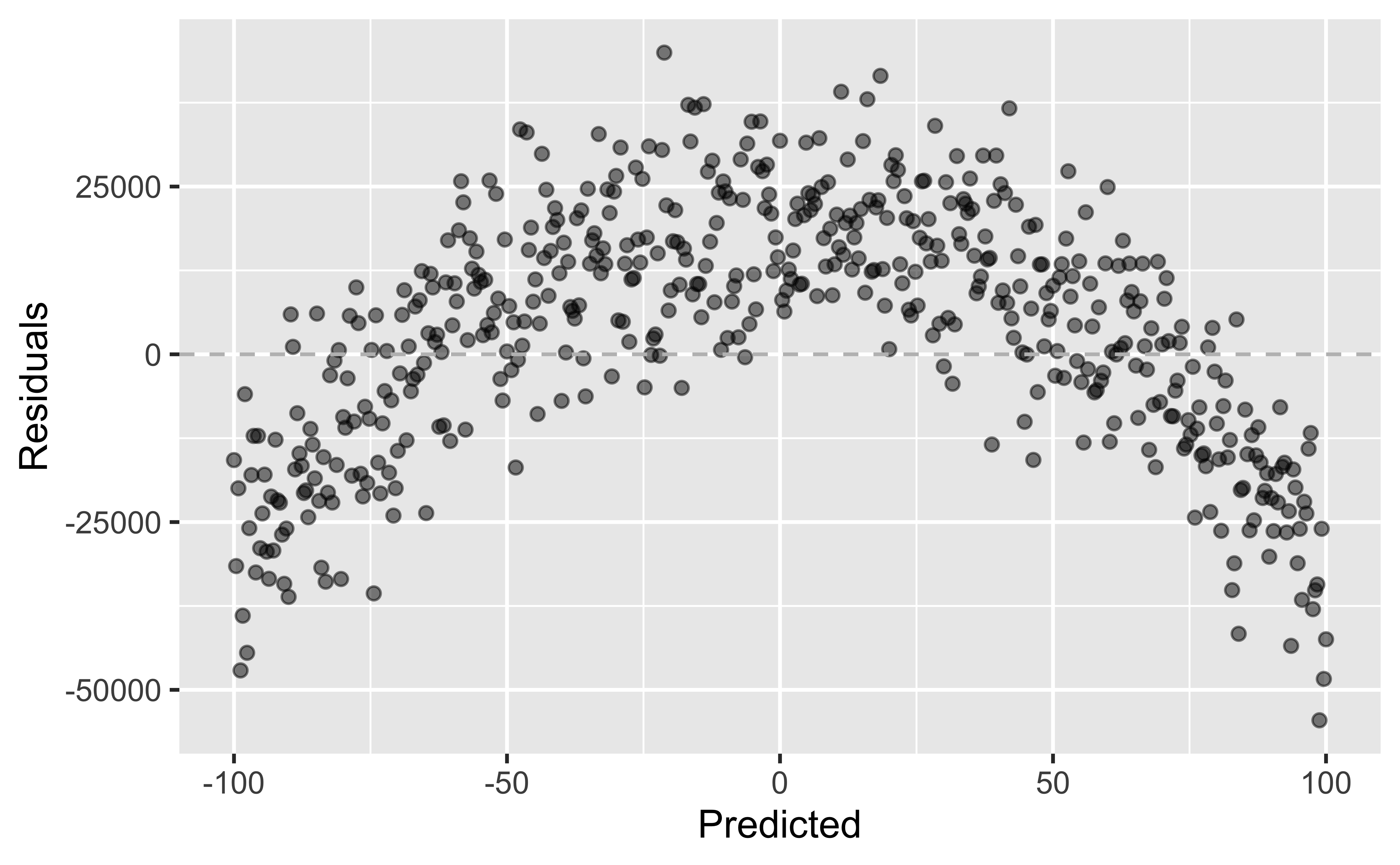
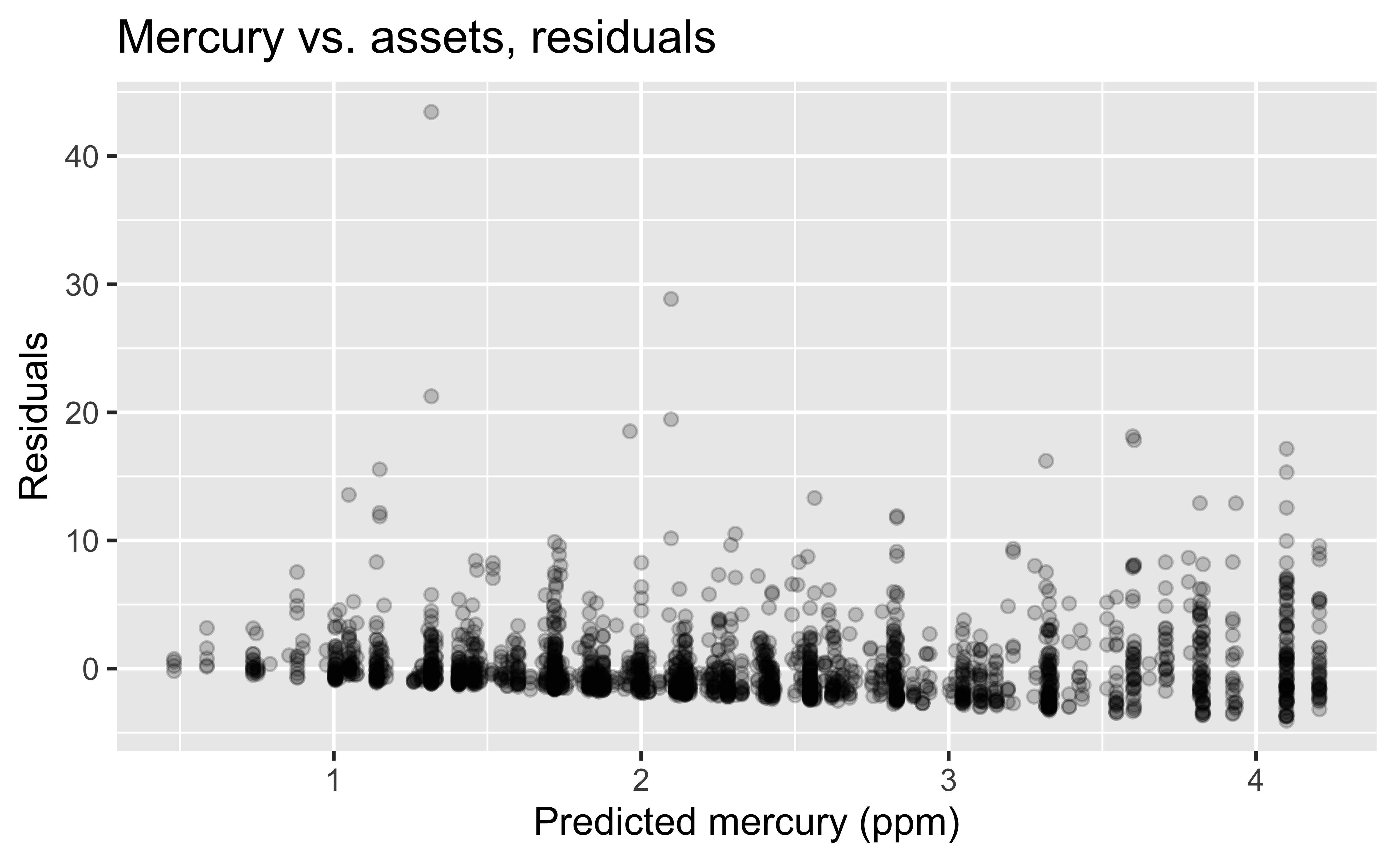
What patterns does the residual plot reveal that should make us question whether a linear model is a good fit for modeling the relationship between mercury (ppm) and assets?
Exploring linearity
Data: Mercury
Mercury vs. assets
Mercury vs assets
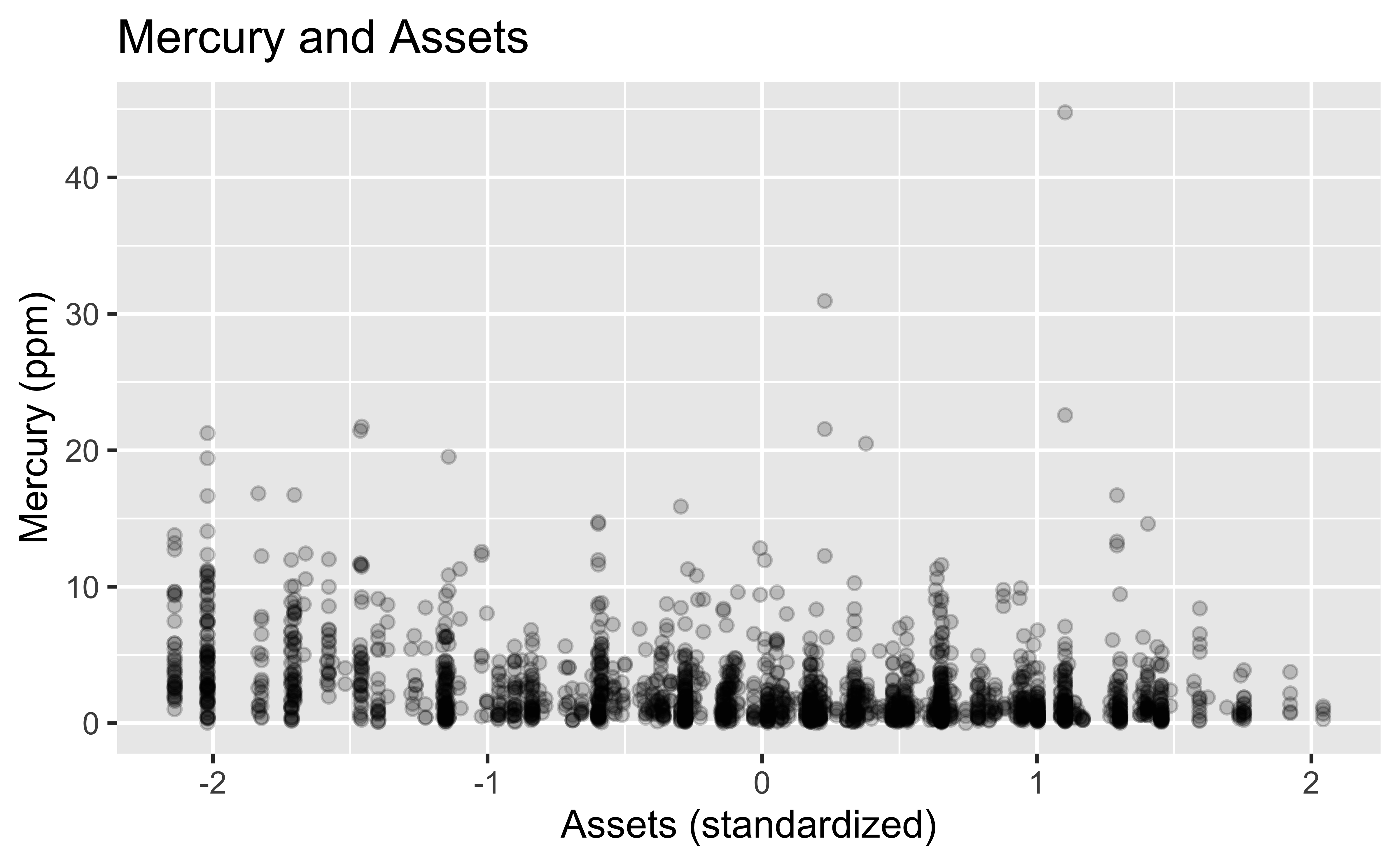
Which plot shows a more linear relationship?
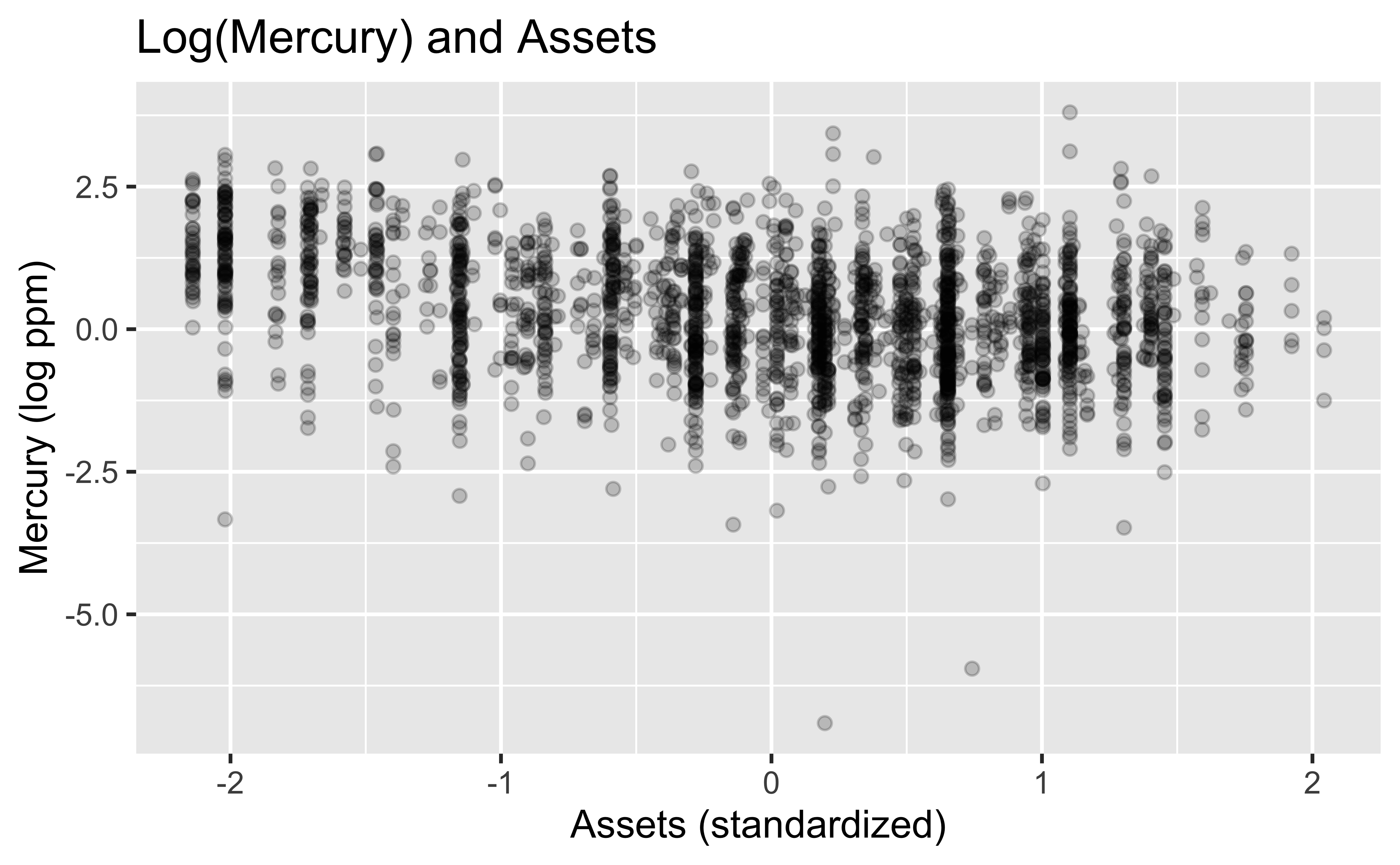
Mercury and Assets, residuals
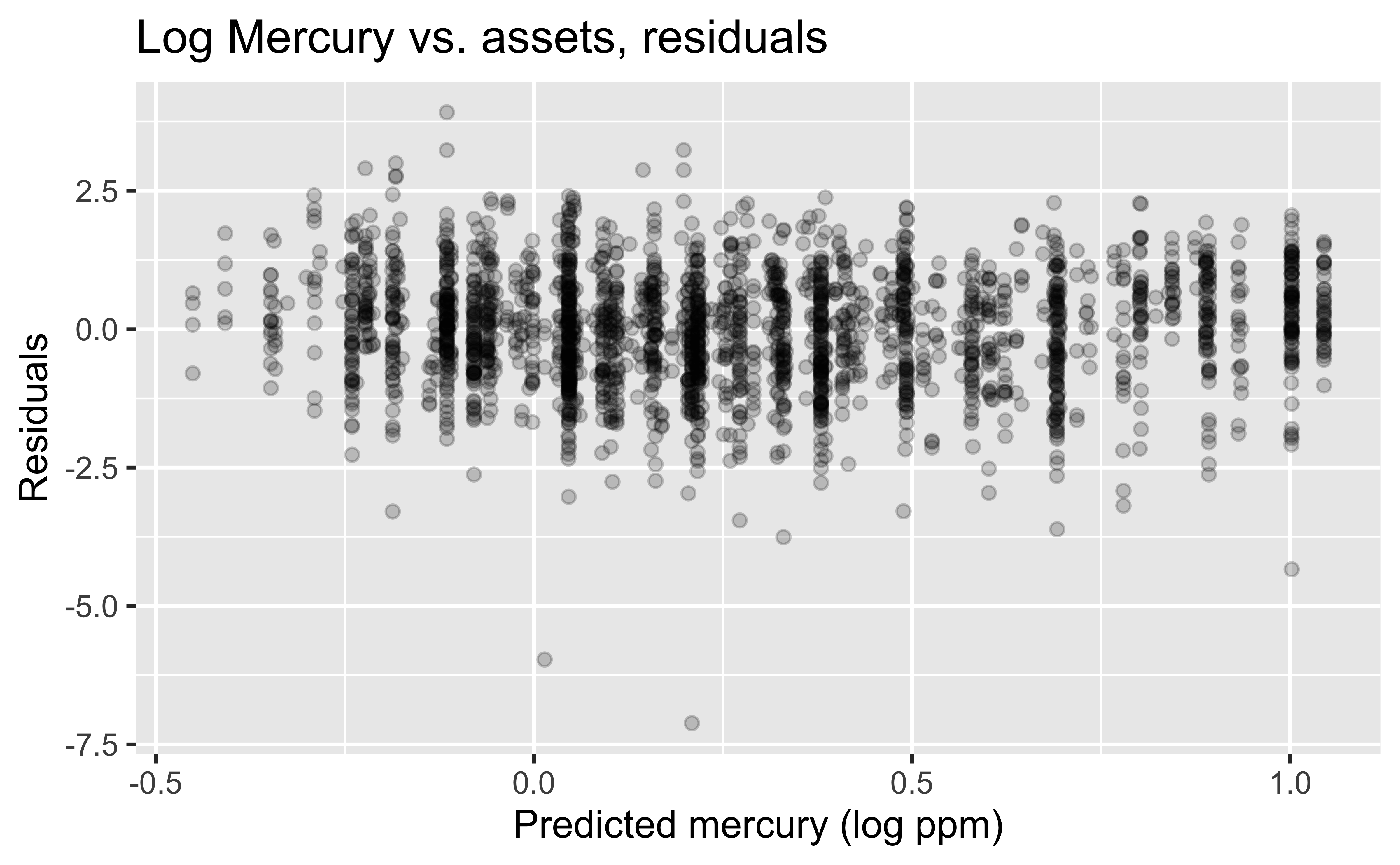
Which plot shows a residuals that are uncorrelated with predicted values from the model? Also, what is the unit of the residuals?
Transforming the data
- We saw that
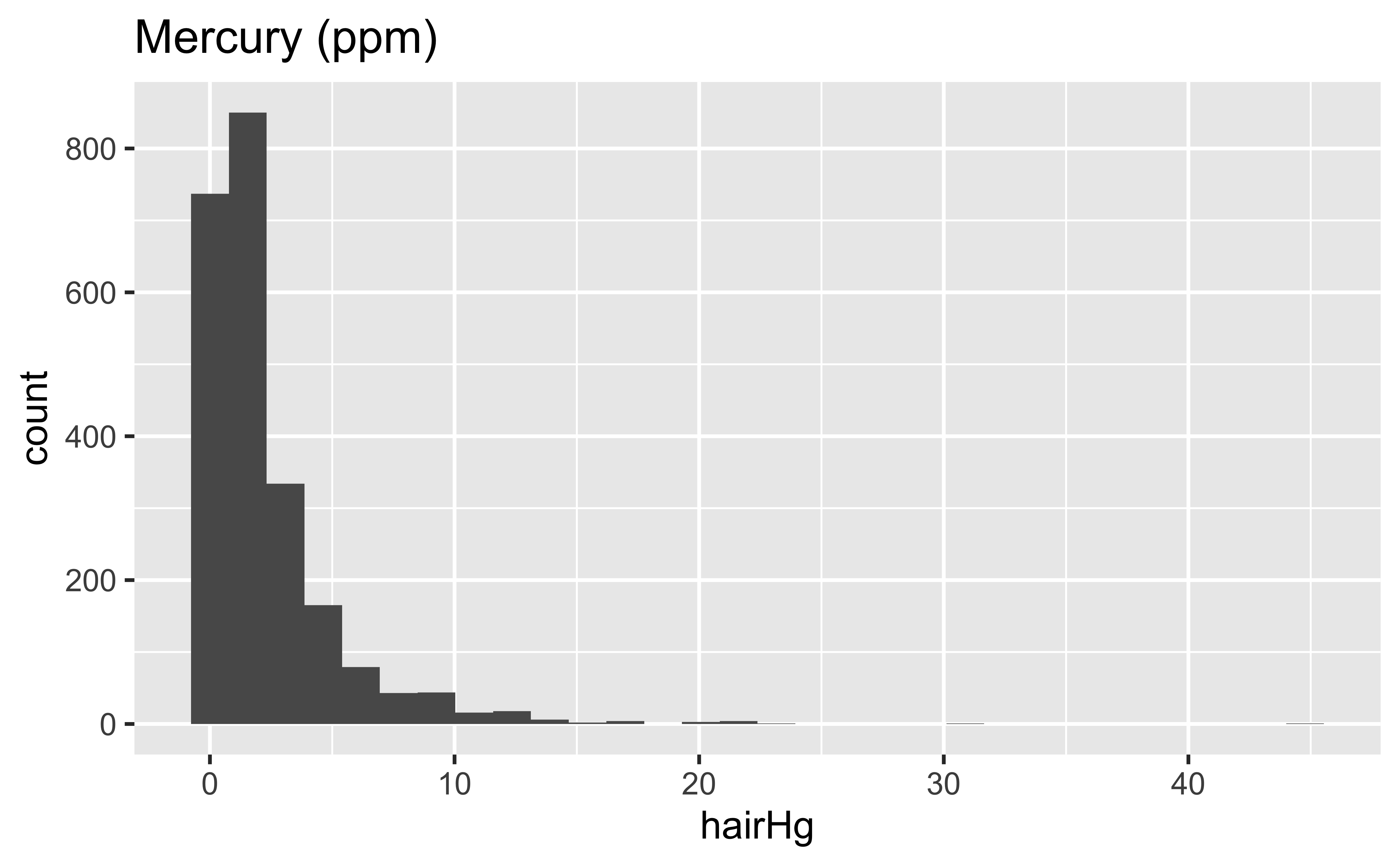
hairHghas a right-skewed distribution, and the residuals of that model don’t look great. - In these situations a transformation applied to the response variable may be useful.
- In order to decide which transformation to use, we should examine the distribution of the response variable.
- The extremely right skewed distribution suggests that a log transformation may be useful.
- log = natural log, \(ln\)
- Default base of the
logfunction in R is the natural log:log(x, base = exp(1))
Transformations
- Non-constant variance is one of the most common model violations, however it is usually fixable by transforming the response (y) variable.
- The most common transformation when the response variable is right skewed is the log transform: \(log(y)\), especially useful when the response variable is (extremely) right skewed.
- This transformation is also useful for variance stabilization.
- When using a log transformation on the response variable the interpretation of the slope changes: “For each unit increase in x, y is expected on average to be higher/lower by a factor of \(e^{\hat{\beta}_1}\).”
- Another useful transformation is the square root: \(\sqrt{y}\), especially useful when the response variable is a count.
Transform, or learn more?
- Data transformations may also be useful when the relationship is non-linear
- However in those cases a polynomial regression may be more appropriate
- This is beyond the scope of this course, but you’re welcomed to try it on your own, and I’d be happy to provide further guidance!
Aside: when \(y = 0\)
In some cases the value of the response variable might be 0, and
log(0)#> [1] -InfThe trick is to add a very small number to the value of the response variable for these cases so that the log function can still be applied:
log(0 + 0.00001)#> [1] -11.51293If there are a lot of 0 values for \(y\), this trick is not such a good idea, and you may need to take an alternative approach (e.g., a zero-inflated model).
Homework (Practice)
- Problem 3
- Problem 4
- Problem 7
- Problem 8
- Problem 12
- Problem 17
- Problem 22
- Problem 23