analysis_births %>%
  count(preterm) %>%
  mutate(percent = scales::percent(n / sum(n), accuracy = 0.1)) %>%
knitr::kable()| preterm | n | percent |
|---|---|---|
| No | 8826 | 88.3% |
| Yes | 1174 | 11.7% |
Introduction to Global Health Data Science
We will use the same 2024 U.S. birth records introduced in the birth weight labs.
How are maternal characteristics associated with birth before 37 completed weeks, called preterm birth?
combgest < 37.This is an analysis of associations in observational data.
The lab used term births only. Here we must include preterm births to study the outcome.
We keep valid gestational ages, maternal ages, and known values of the predictors. Unknown smoking status, BMI, and gestational diabetes status are excluded. We draw a new sample of 10,000 births; the earlier lab’s term-only sample cannot answer this question.
| Variable | In the data | In our analysis |
|---|---|---|
| Gestational age | combgest |
preterm: Yes if less than 37 weeks |
| Maternal age | mager |
<15, 15–39, or 40+ years |
| Pre-pregnancy BMI | bmi_r |
Underweight (<18.5), normal (18.5–24.9), overweight (25–29.9), obese (≥30) |
| Smoking during pregnancy | cig_rec |
smoking: No or Yes |
| Gestational diabetes | rf_gdiab |
gest_diabetes: No or Yes |
| Plurality | dplural |
Singleton or multiple birth |
bmi_r measures pre-pregnancy BMI; its three obesity codes are combined here. Ages 40 and above are in 40+, so the middle group ends at 39.
A birth at 37 completed weeks belongs to the term birth group.
analysis_births %>%
count(preterm) %>%
mutate(percent = scales::percent(n / sum(n), accuracy = 0.1)) %>%
knitr::kable()| preterm | n | percent |
|---|---|---|
| No | 8826 | 88.3% |
| Yes | 1174 | 11.7% |
Which outcome should we code as the event of interest? Here Yes is the second factor level, so the fitted model targets the probability of preterm birth.
analysis_births %>%
  ggplot(aes(x = smoking, fill = preterm)) +
  geom_bar(position = "fill") +
  scale_y_continuous(labels = scales::label_percent()) +
  scale_fill_manual(values = c("No" = "#B9AEC8", "Yes" = "#012169")) +
  labs(x = "Smoking during pregnancy", y = "Proportion of births",
       fill = "Preterm")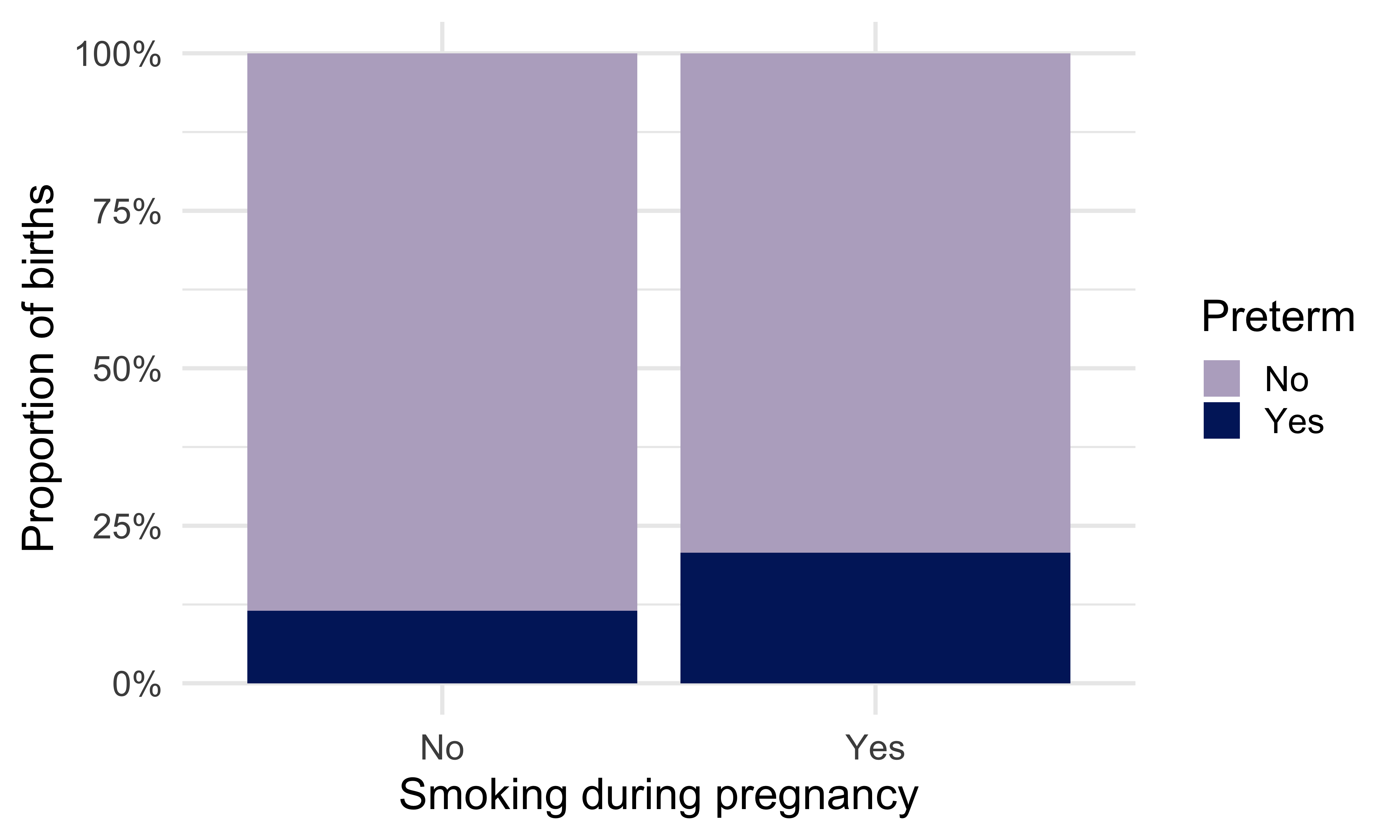
analysis_births %>%
  ggplot(aes(x = gest_diabetes, fill = preterm)) +
  geom_bar(position = "fill") +
  scale_y_continuous(labels = scales::label_percent()) +
  scale_fill_manual(values = c("No" = "#B9AEC8", "Yes" = "#012169")) +
  labs(x = "Gestational diabetes", y = "Proportion of births",
       fill = "Preterm")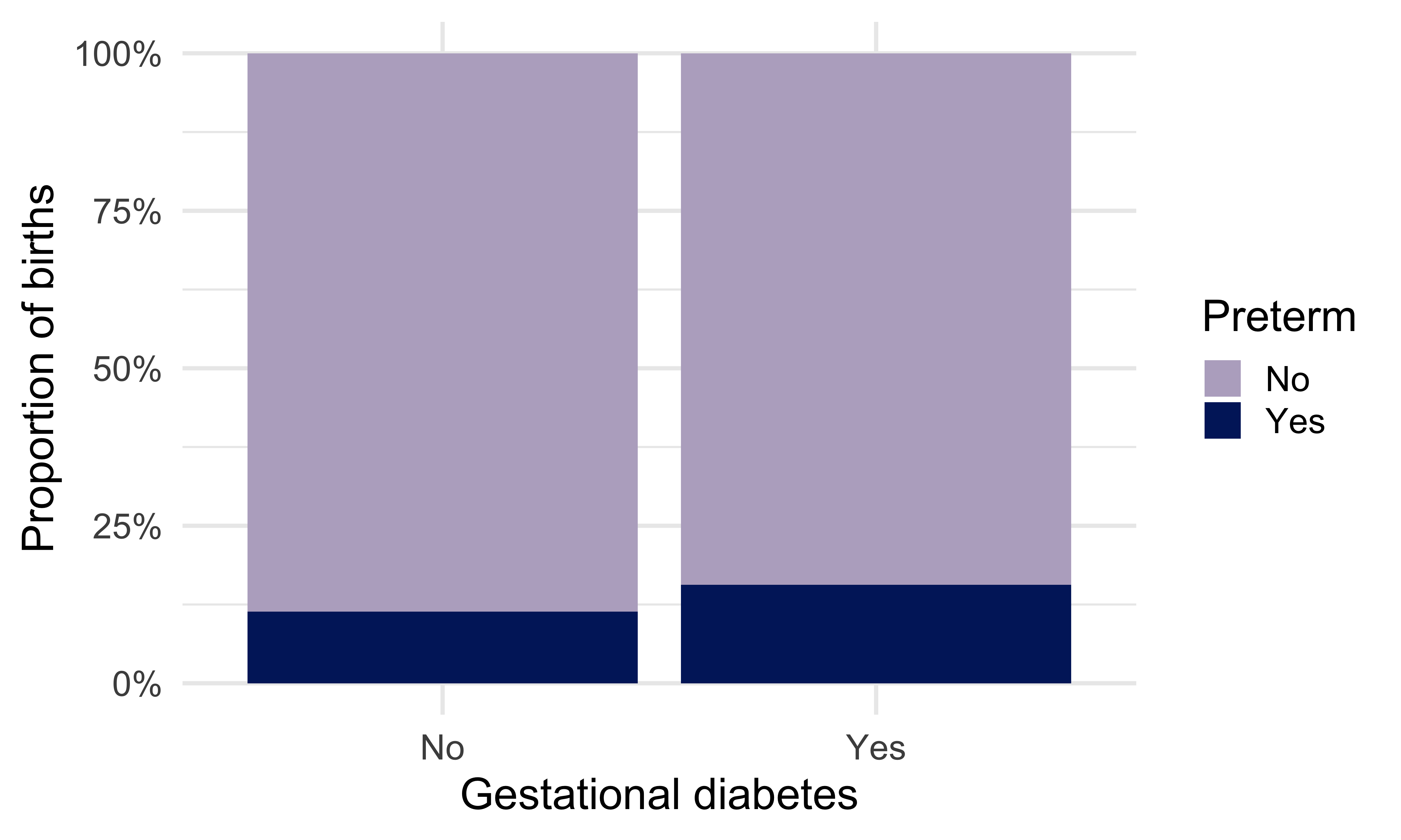
analysis_births %>%
  ggplot(aes(x = plurality, fill = preterm)) +
  geom_bar(position = "fill") +
  scale_y_continuous(labels = scales::label_percent()) +
  scale_fill_manual(values = c("No" = "#B9AEC8", "Yes" = "#012169")) +
  labs(x = "Plurality", y = "Proportion of births", fill = "Preterm")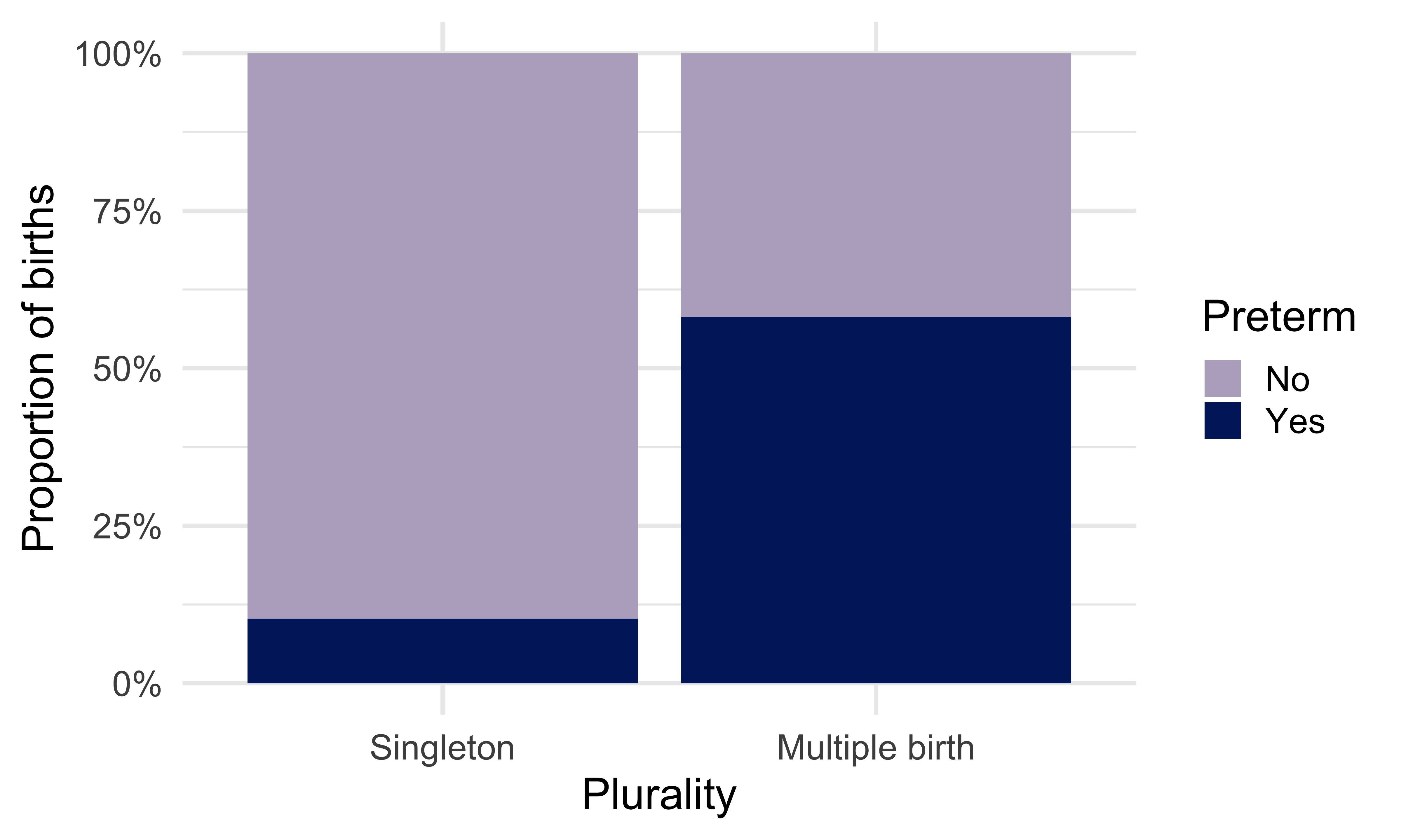
analysis_births %>%
  ggplot(aes(x = bmi_category, fill = preterm)) +
  geom_bar(position = "fill") +
  scale_x_discrete(limits = c("Underweight", "Normal", "Overweight", "Obese")) +
  scale_y_continuous(labels = scales::label_percent()) +
  scale_fill_manual(values = c("No" = "#B9AEC8", "Yes" = "#012169")) +
  labs(x = "Pre-pregnancy BMI category", y = "Proportion of births",
       fill = "Preterm")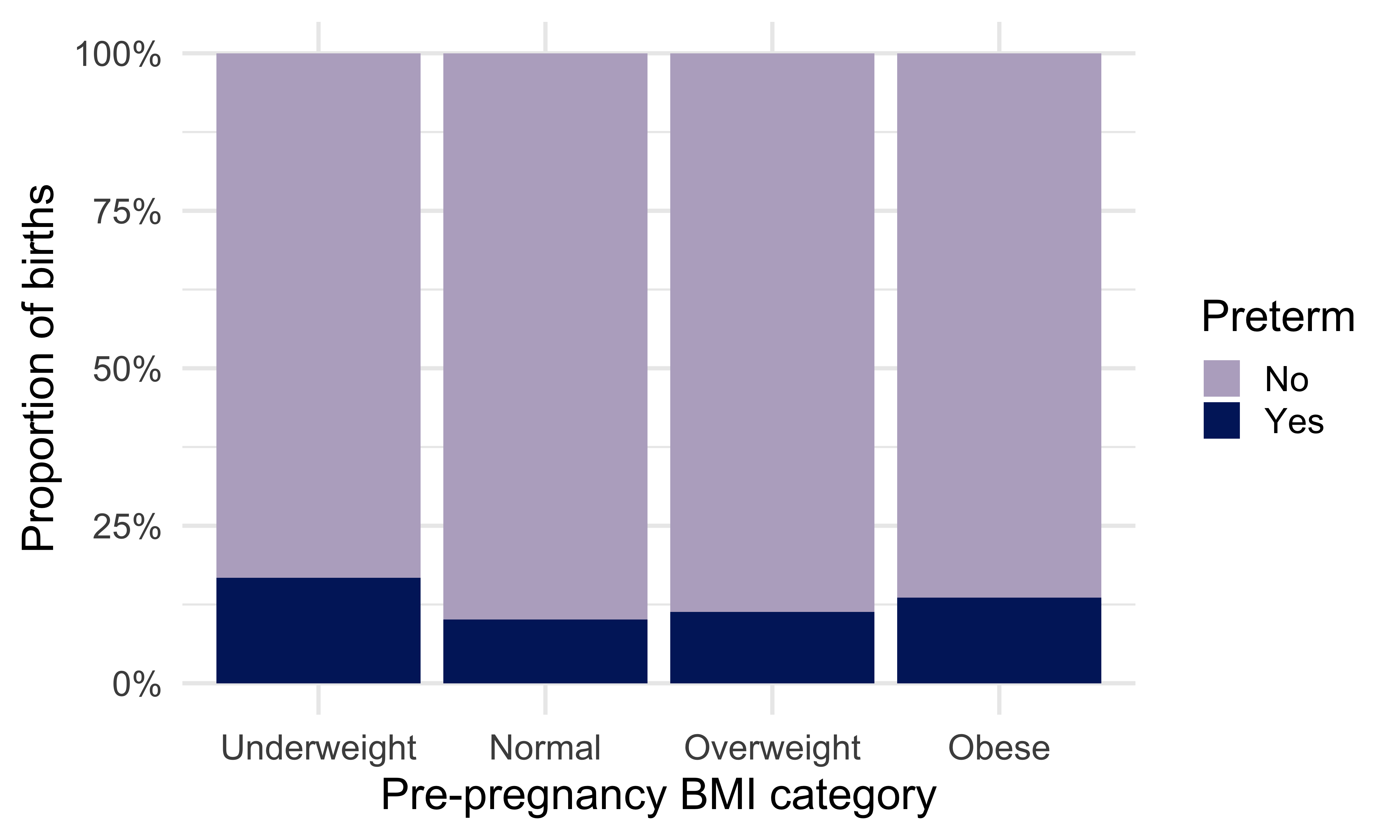
analysis_births %>%
  ggplot(aes(x = age_group, fill = preterm)) +
  geom_bar(position = "fill") +
  scale_x_discrete(limits = c("<15", "15-39", "40+")) +
  scale_y_continuous(labels = scales::label_percent()) +
  scale_fill_manual(values = c("No" = "#B9AEC8", "Yes" = "#012169")) +
  labs(x = "Maternal age group (years)", y = "Proportion of births",
       fill = "Preterm")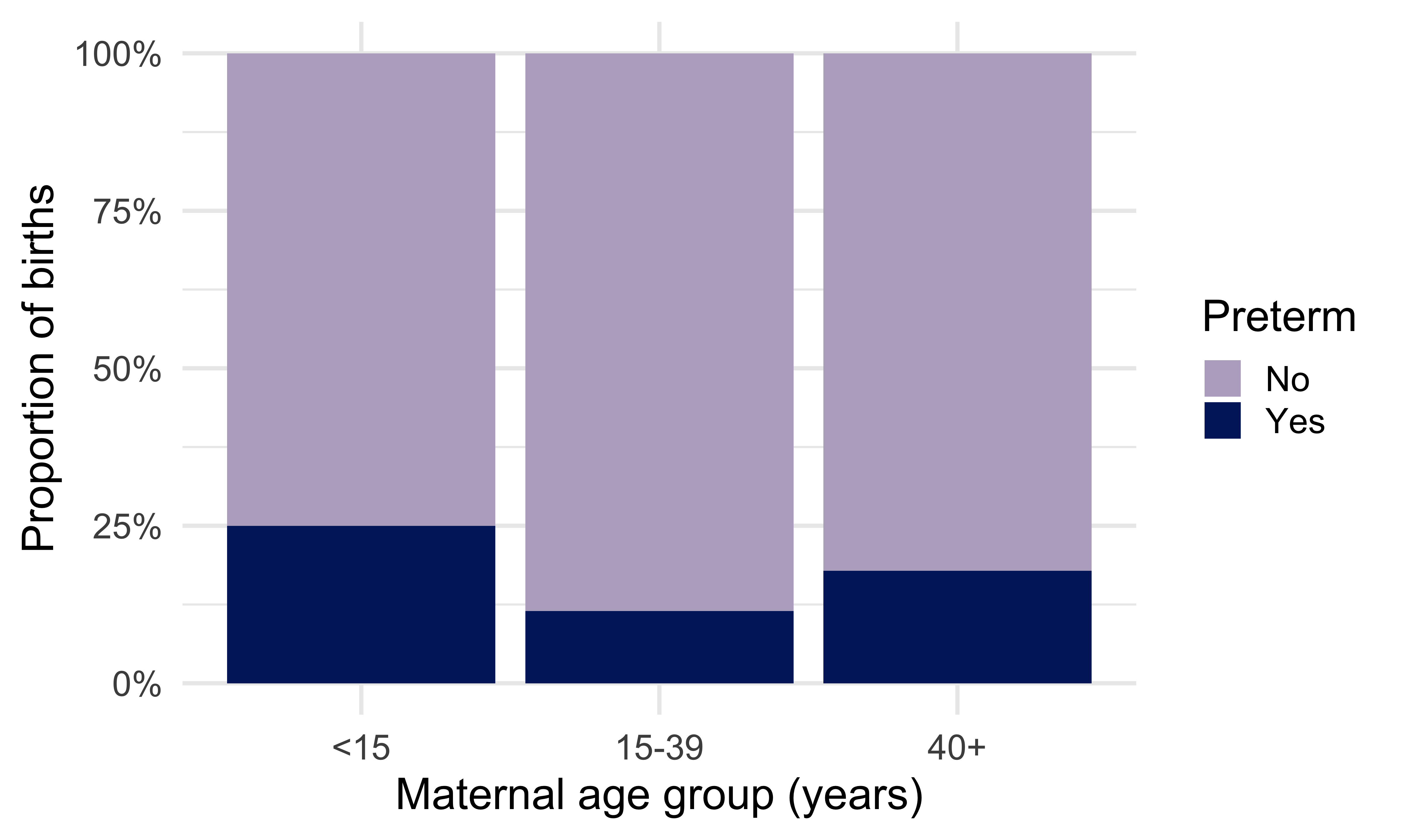
Question: Why can we describe associations from these plots but not infer that a predictor caused a preterm birth?
For birth \(i\), define
\[Y_i=\begin{cases}1 & \text{if gestational age is less than 37 weeks},\\ 0 & \text{otherwise.}\end{cases}\]
Each \(Y_i\) has two possible values. We can model it with a Bernoulli distribution:
\[Y_i\sim\operatorname{Bernoulli}(\pi_i),\qquad \pi_i=P(Y_i=1\mid X_i).\]
The probability \(\pi_i\) can depend on the birth’s predictors \(X_i\). This relaxes our assumption about previous binomial data, in which everyone needed to have the same probability \(\pi\) of the outcome.
If we model \(\pi_i\) directly with a straight line, a prediction could be less than 0 or greater than 1.
We need a model that permits a linear combination of predictors and produces valid probabilities between 0 and 1.
Logistic regression connects the linear predictor to the probability through the logit function.
Outcome distribution: \(Y_i\sim\operatorname{Bernoulli}(\pi_i)\).
Linear predictor: \(\eta_i=\beta_0+\beta_1 X_{1i}+\cdots+\beta_k X_{ki}\).
Link function: \(\operatorname{logit}(\pi_i)=\eta_i\).
Ordinary linear regression also has these three pieces, but uses a normal distribution and the identity link.
For an event with probability \(\pi\):
\[\text{odds}=\frac{\pi}{1-\pi},\qquad \operatorname{logit}(\pi)=\log\left(\frac{\pi}{1-\pi}\right).\]
The logit is defined for \(0<\pi<1\).
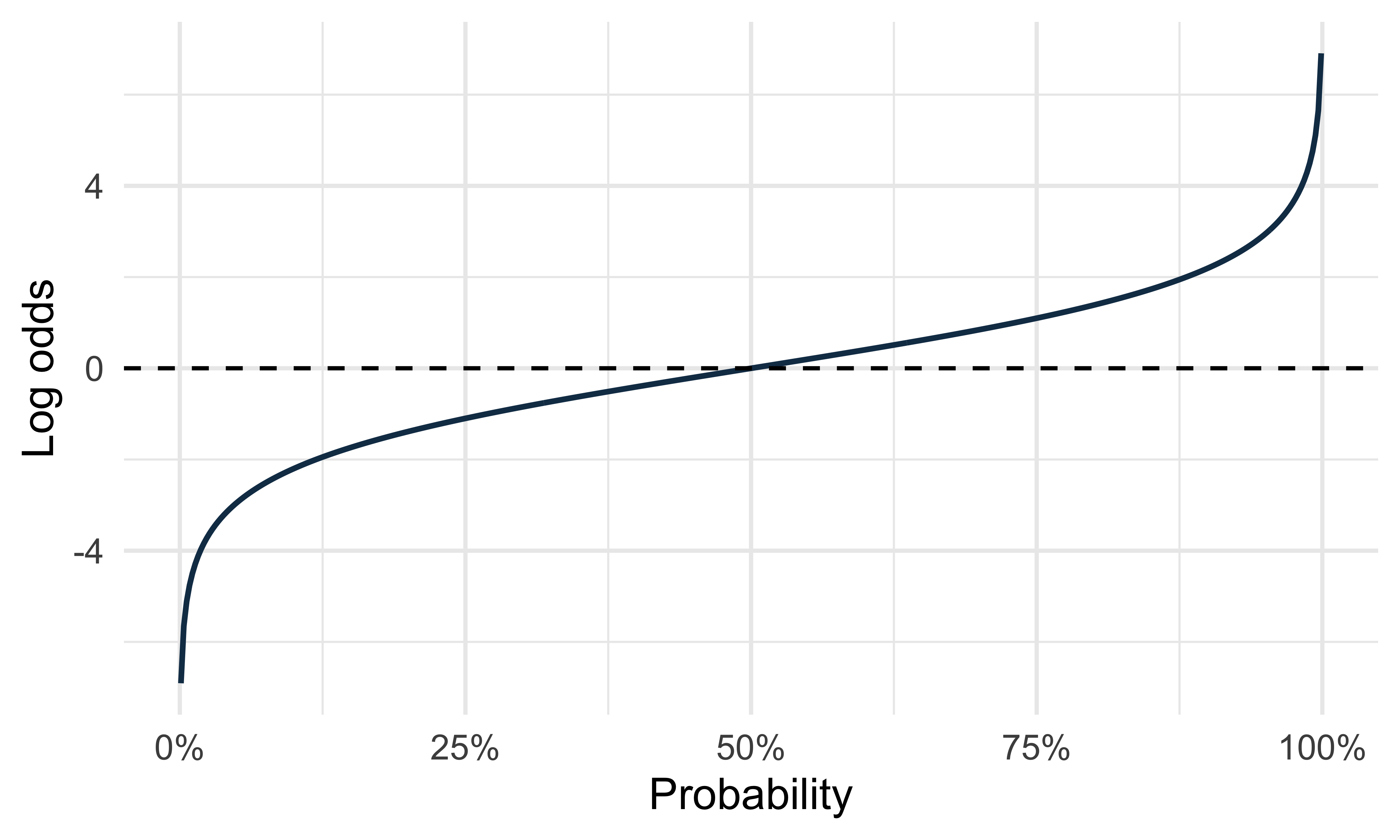
The inverse logit converts any linear predictor \(\eta_i\) into a probability:
\[\pi_i=\frac{\exp(\eta_i)}{1+\exp(\eta_i)} =\frac{1}{1+\exp(-\eta_i)}.\]
When \(\eta_i=0\), the probability is \(0.5\). A positive value produces a probability above \(0.5\); a negative value produces a probability below \(0.5\).
An indicator variable records whether a condition is true (1) or false (0). For example,
\[ I(\text{maternal age}<15)= \begin{cases} 1 & \text{if the mother is younger than 15},\\ 0 & \text{if the mother is 15 or older}. \end{cases} \]
| Maternal age | \(I(\text{age}<15)\) |
|---|---|
| 14 | 1 |
| 15 | 0 |
| 25 | 0 |
| 45 | 0 |
\[ I(\text{maternal age}>40)= \begin{cases} 1 & \text{if the mother is older than 40},\\ 0 & \text{if the mother is 40 or younger}. \end{cases} \]
| Maternal age | \(I(\text{age}\ge40)\) |
|---|---|
| 14 | 0 |
| 15 | 0 |
| 25 | 0 |
| 45 | 1 |
So looking at both indicator variables together, we understand the age group of the participant.
| Maternal age | \(I(\text{age}<15)\) | \(I(\text{age}\ge40)\) |
|---|---|---|
| 14 | 1 | 0 |
| 15 | 0 | 0 |
| 25 | 0 | 0 |
| 45 | 0 | 1 |
In a logistic regression, the indicator lets us compare mothers under 15 with the reference group, mothers 15-39. Its exponentiated coefficient is the odds ratio for that comparison. Similarly, we can also compare older mothers to the reference group.
Use ages 15–39 as the reference group. The model adds one indicator for ages under 15 and another for ages 40 or older:
\[\operatorname{logit}(\pi_i)=\beta_0 +\beta_1 I(\text{age}<15)_i +\beta_2 I(\text{age}\ge40)_i.\]
The intercept \(\beta_0\) is the log odds of preterm birth for the 15–39 group. We call this model an unadjusted model because it only assesses the effects of a single predictor, maternal age.
age_fit <- logistic_reg() %>%
  set_engine("glm") %>%
  fit(preterm ~ age_group, data = analysis_births)

tidy(age_fit, conf.int = TRUE) %>%
  mutate(across(where(is.numeric), ~round(.x, 3))) %>%
knitr::kable()| term | estimate | std.error | statistic | p.value | conf.low | conf.high |
|---|---|---|---|---|---|---|
| (Intercept) | -2.046 | 0.032 | -63.631 | 0.000 | -2.110 | -1.984 |
| age_group<15 | 0.948 | 1.155 | 0.820 | 0.412 | -2.059 | 3.004 |
| age_group40+ | 0.519 | 0.127 | 4.096 | 0.000 | 0.265 | 0.762 |
The model estimates one coefficient for under 15 versus 15–39 and another for 40+ versus 15–39.
The fitted odds for ages 15–39 and 40+ are
\[\text{odds}_{15\text{–}39}=\exp(\beta_0),\qquad \text{odds}_{40+}=\exp(\beta_0+\beta_2).\]
Thus \(\exp(\beta_2)\) is the odds ratio for 40+ versus 15–39. Similarly, \(\exp(\beta_1)\) compares under 15 versus 20–39.
These comparisons are for groups, rather than for a one-year or ten-year difference.
The two coefficient tests ask separate questions:
The test used is based on a \(z\)-score constructed by taking our estimate, subtracting 0, and then dividing by the standard deviation of our estimate.
Exponentiating each coefficient and its confidence limits gives the odds ratio and its confidence interval for that comparison.
tidy(age_fit, conf.int = TRUE, exponentiate = TRUE) %>%
  filter(term != "(Intercept)") %>%
  select(term, estimate, conf.low, conf.high, p.value) %>%
  mutate(across(where(is.numeric), ~round(.x, 3))) %>%
knitr::kable()| term | estimate | conf.low | conf.high | p.value |
|---|---|---|---|---|
| age_group<15 | 2.579 | 0.128 | 20.166 | 0.412 |
| age_group40+ | 1.680 | 1.303 | 2.142 | 0.000 |
The usual model standard errors treat birth records as independent; births from the same multiple pregnancy will violate this assumption.
| term | estimate | conf.low | conf.high | p.value |
|---|---|---|---|---|
| age_group<15 | 2.579 | 0.128 | 20.166 | 0.412 |
| age_group40+ | 1.680 | 1.303 | 2.142 | 0.000 |
Mothers aged \(<15\) do not have significantly different risk of preterm birth as mothers aged 15-39. Mothers aged 40+ have 1.68 (1.30, 2.14) times the odds of preterm birth as their counterparts aged 15-39.
Now include the five predictors. We call this type of model a multiple logistic regression model or an adjusted model. The age and BMI categories enter the model through indicator variables:
\[ \begin{aligned} \log\left(\frac{\pi_i}{1-\pi_i}\right) ={}& \beta_0 +\beta_1 I(\text{age}_i<15) +\beta_2 I(\text{age}_i\ge 40)\\ &+\beta_3 I(\text{BMI}_i=\text{Underweight}) +\beta_4 I(\text{BMI}_i=\text{Overweight})\\ &+\beta_5 I(\text{BMI}_i=\text{Obese}) +\beta_6 I(\text{smoking}_i=\text{Yes})\\ &+\beta_7 I(\text{gestational diabetes}_i=\text{Yes}) +\beta_8 I(\text{plurality}_i=\text{Multiple birth}). \end{aligned} \]
Reference group: ages 15–39, normal BMI, no smoking, no gestational diabetes, and singleton.
birth_fit <- logistic_reg() %>%
  set_engine("glm") %>%
  fit(preterm ~ age_group + bmi_category + smoking +
        gest_diabetes + plurality,
      data = analysis_births)
We use exponentiate = TRUE to turn the coefficients into odds ratios. Each estimate compares one category with its reference category while holding the other predictors fixed.
tidy(birth_fit, conf.int = TRUE, exponentiate = TRUE) %>%
  filter(str_starts(term, "age_group") |
           str_starts(term, "bmi_category")) %>%
  select(term, estimate, conf.low, conf.high, p.value) %>%
  mutate(across(where(is.numeric), ~round(.x, 3))) %>%
knitr::kable()| term | estimate | conf.low | conf.high | p.value |
|---|---|---|---|---|
| age_group<15 | 3.427 | 0.169 | 26.845 | 0.287 |
| age_group40+ | 1.615 | 1.238 | 2.083 | 0.000 |
| bmi_categoryUnderweight | 1.858 | 1.265 | 2.663 | 0.001 |
| bmi_categoryOverweight | 1.139 | 0.966 | 1.342 | 0.122 |
| bmi_categoryObese | 1.335 | 1.145 | 1.556 | 0.000 |
Each age-group estimate compares with ages 15–39. Each BMI estimate compares with normal pre-pregnancy BMI. For each comparison, we assume no other predictor values change.
| term | estimate | conf.low | conf.high | p.value |
|---|---|---|---|---|
| age_group<15 | 3.427 | 0.169 | 26.845 | 0.287 |
| age_group40+ | 1.615 | 1.238 | 2.083 | 0.000 |
| bmi_categoryUnderweight | 1.858 | 1.265 | 2.663 | 0.001 |
| bmi_categoryOverweight | 1.139 | 0.966 | 1.342 | 0.122 |
| bmi_categoryObese | 1.335 | 1.145 | 1.556 | 0.000 |
Mothers aged 40+ have 1.62 (1.24, 2.08) times the odds of preterm birth as mothers aged 15-39, adjusting for BMI, smoking status, gestational diabetes status, and plurality. Underweight mothers have 1.86 (1.27, 2.66) times the odds of preterm birth as their normal weight counterparts, and obese mothers have 1.34 (1.15, 1.56) times the odds of preterm birth as their normal weight counterparts, adjusting for maternal age, smoking status, gestational diabetes status, and plurality. Thus both age and BMI are predictors of the probability of preterm birth.
tidy(birth_fit, conf.int = TRUE, exponentiate = TRUE) %>%
  filter(term != "(Intercept)",
         !str_starts(term, "age_group"),
         !str_starts(term, "bmi_category")) %>%
  select(term, estimate, conf.low, conf.high, p.value) %>%
  mutate(across(where(is.numeric), ~round(.x, 3))) %>%
knitr::kable()| term | estimate | conf.low | conf.high | p.value |
|---|---|---|---|---|
| smokingYes | 1.893 | 1.355 | 2.598 | 0.000 |
| gest_diabetesYes | 1.346 | 1.091 | 1.650 | 0.005 |
| pluralityMultiple birth | 12.013 | 9.480 | 15.264 | 0.000 |
For example, smokingYes compares reported smoking with no smoking among births with the same age group, BMI category, diabetes status, and plurality.
| term | estimate | conf.low | conf.high | p.value |
|---|---|---|---|---|
| smokingYes | 1.893 | 1.355 | 2.598 | 0.000 |
| gest_diabetesYes | 1.346 | 1.091 | 1.650 | 0.005 |
| pluralityMultiple birth | 12.013 | 9.480 | 15.264 | 0.000 |
Maternal smoking, gestational diabetes, and higher-order pregnancies also convey greater risk of preterm birth. Women smoking during pregnancy have 1.89 (1.36, 2.60) times the odds of preterm birth as their nonsmoking counterparts, after adjustment for maternal age, BMI, gestational diabetes status, and the multiplicity of the pregnancy. Similarly, gestational diabetes is associated with 1.35 (1.09, 1.65) times the odds of preterm birth, and a multiple pregnancy is associated with a whopping 12.0 (9.5, 15.3) times the odds of preterm birth, after adjusting for the other factors in the model.
Simple (unadjusted) model
\[ \begin{aligned} \operatorname{logit}\{P(Y_i=1\mid X_i)\} &= \alpha_0+\alpha_1X_i. \end{aligned} \]
For a one-unit increase in \(X\), the estimated crude odds ratio is
\[ \widehat{OR}_{\text{crude}}=e^{\hat{\alpha}_1}. \]
Multiple (adjusted) model
\[ \begin{aligned} \operatorname{logit}\{P(Y_i=1\mid X_i,\mathbf Z_i)\} &= \beta_0+\beta_1X_i\\ &\quad+\beta_2Z_{2i}+\cdots+\beta_pZ_{pi}. \end{aligned} \]
Holding the other predictors constant, the estimated adjusted odds ratio is
\[ \widehat{OR}_{\text{adjusted}}=e^{\hat{\beta}_1}. \]
The two odds ratios answer different questions.
Crude OR: How do the odds of \(Y=1\) compare for groups that differ by one unit in \(X\), without accounting for other predictors?
Adjusted OR: How do the odds compare for groups that differ by one unit in \(X\) but have the same values of the other predictors?
For binary \(X\), this compares \(X=1\) with \(X=0\).
The adjusted interpretation assumes the model does not include interactions involving \(X\).
A confounder is a variable that creates a noncausal association between the predictor of interest and the outcome.
For example, a third variable \(Z\) may influence both \(X\) and \(Y\):
\[ X \leftarrow Z \rightarrow Y. \]
Subject-matter knowledge helps us decide which variables to adjust for.
Confounding can make an association appear stronger, weaker, or even point in the opposite direction.
| Pattern | What can happen after appropriate adjustment? |
|---|---|
| Crude association exaggerated | The OR moves closer to 1. |
| Crude association masked | The OR moves further from 1. |
| Crude association reversed | The OR changes from above 1 to below 1, or vice versa. |
A reversal between an overall association and associations within subgroups is an example of Simpson’s paradox.
A change in the estimated OR alone does not establish that a variable is a confounder.
Suppose \(Z\) influences both \(X\) and \(Y\).
For each observation \(i=1,\ldots,n\):
\[ \begin{aligned} Z_i &\sim \operatorname{Bernoulli}(0.5),\\[6pt] \operatorname{logit}\!\left\{P(X_i=1\mid Z_i)\right\} &= -1+2Z_i,\\[6pt] \operatorname{logit}\!\left\{P(Y_i=1\mid X_i,Z_i)\right\} &= -1+0.5X_i+1.5Z_i. \end{aligned} \]
Here, \(X_i\) and \(Y_i\) are binary, and \(\operatorname{logit}(p)=\log\{p/(1-p)\}\).
Thus, \(Z\) predicts both \(X\) and \(Y\), while \(X\) also predicts \(Y\).
or_confounding_simple <- logistic_reg() %>%
  set_engine("glm") %>%
  fit(y ~ x, data = or_confounding_data)

or_confounding_adjusted <- logistic_reg() %>%
  set_engine("glm") %>%
fit(y ~ x + z, data = or_confounding_data)| Model | Estimated OR | 95% CI: lower | 95% CI: upper |
|---|---|---|---|
| Crude | 3.042 | 2.872 | 3.223 |
| Adjusted | 1.645 | 1.540 | 1.757 |
Both models use the same observations.
The simulation was constructed so that \(Z\) influences both \(X\) and \(Y\).
For this data-generating mechanism, the population crude OR is approximately 3.05, compared with the conditional OR of 1.65.
The simulated estimates will vary around these values.
Compare the same observations. Added predictors may have missing values, causing the adjusted model to use a smaller sample.
Use subject-matter knowledge. Decide whether a variable could create a noncausal association between \(X\) and \(Y\).
Interpret the adjusted OR conditionally. State which variables are being held constant.
Avoid causal conclusions from adjustment alone. Including additional predictors does not automatically make an association causal.